Incremental_Backward_Change_Propagation_of_View_Models_by_Logic_Solvers

!Currently Under Construction!

This page is dedicated to the measurement results of the research paper "Incremental Backward Change Propagation of View Models by Logic Solvers". For more information please write to semerath@mit.bme.hu.

In order to evaluate the performance of the key step of our backward change propagation technique we have conducted initial measurements on a prototype implementation in the context of the running example as case study (taken from the CONCERTO project). Our evaluation exclusively focuses on assessing the performance of the model generation step for the source model (detailed in Sec. 3.3), and excludes the performance evaluation of change partitioning (Sec. 3.2). In our initial experiments, we experienced that both the change partitioning time (i.e. the selection of affected source elements) and the forward transformation time is negligible (less than 1 second for the largest problems we measured) compared to the time required to solve the logic problem by Alloy. Thus performance limitations are dominated by the latter.

Change propagation problem generator

In order to measure the performance of our technique we extended the running example of the paper to a change propagation benchmark, which can be parametrized and scaled by the size (s) of the source model and the number of changes (c) in the views. We have created valid health care models in the following five steps:

• 1. First, a Sensor is created with a PeriodicTrigger.
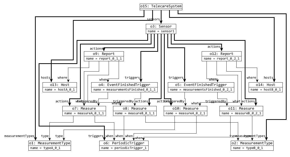
• 2. Two MeasurementTypes are added to the model, which are measured by two respective Measures activated by the periodic trigger. Then two Reports are added to the model, which are triggered by two new EventFinishedTriggers waiting for the measurements of two different types. Then the result is reported to two newly created Hosts.
• 3. Step 2 is repeated s times, which means that the model has 2×s MeasurementTypes, 4×s Measures, 2×s Reports, 2×s EventFinishedTriggers and 2×s Hosts.

There are some illustrations for the generated source models for three different sizes:

<tr><td>2</td>
  <td>
    <img alt="" src="https://raw.githubusercontent.com/wiki/FTSRG/publication-pages/bx_modelgenerator/Illustrations/original_s2.png">
  </td>
</tr>

<tr><td>3</td>
  <td>
    <img alt="" src="https://raw.githubusercontent.com/wiki/FTSRG/publication-pages/bx_modelgenerator/Illustrations/original_s3.png">
  </td>
</tr>

s	Original Source Model
1

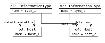
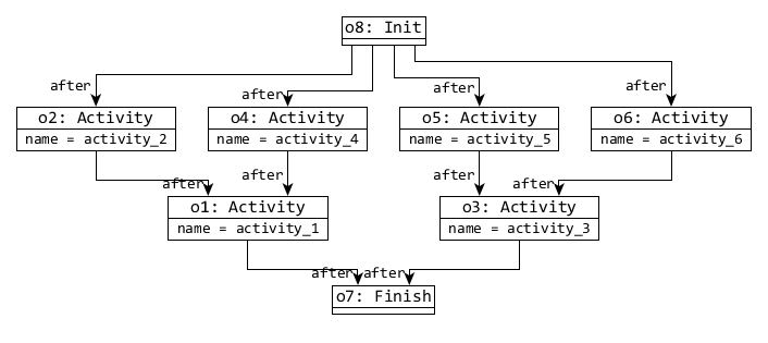
• 4. The view models are derived, which creates in a dataflow model with 2×s Hosts and 2×s InformationTypes 4×s dataflow references, and an event ordering model with 1 Init, 1 Finish, 6×s Activities and 10×s after references.

Therefore the previously mentioned models are transformed to the following view models:

s	Dataflow view	Event Ordering view
1
2
3

• 5. Then finally, changes are applied to the view models: c MeasurementType and c Hosts with their dataflow references are randomly removed from the first view model, and a new Action is added to the event ordering view.

There are two size 2 models with c=1 and c=2, where red model elements are removed, and green are created by the change:

c	Dataflow view	Event Ordering view
1
2

As a result, we obtain non-trivial source and view models, while the random changes of the view model remain semantically meaningful.

Measurement Setup

Each model generation task was executed on the generated healthcare change propagation problems using the Alloy Analyzer with SAT4j-solver (available at the link). Each change propagation problem is solved with our incremental solution which generates only the affected part in the source model. As a baseline, we compare it to a solution which generates full models for a view model. The full model generation is achieved as a corner case of the incremental generation where the changed view models are interpreted as if they were newly created, and no part of the source model is preserved.

We measured the runtime of Alloy Analyzer, which consists of an initial conversion to a conjunctive normal form and then solving the SAT-problem by the back-end solver. We executed each measurement 5 times, then the average of the execution times was calculated. The measurements were executed with a 120 second timeout on an average personal computer.

Measurement Cases

For the sake of reproducability, we uploaded the cases presented in the paper.

• This file contains results measured by us.
• This archive contains the measurement cases we checked. The structure of the archive is the following:
  • In the root there is folder called *Incremental", which contains the incremental cases, and an AllInOne folder where the whole source model is regenerated.
  • Those folders contains the measurement scenario subfolders with "s,c" names, where s marks the size of the model, c marks the number of changes.
  • Each scenario folder contains the following documents:
    • experiment-original.gml contains the visual representation of the original source model.
    • experiment-dataflow-original.gml contains the visual representation of the original Dataflow view.
    • experiment-events-original.gml contains the visual representation of the original Event Ordering view.
    • experiment-dataflow-modified.gml contains the visual representation of the changed Dataflow view.
    • experiment-events-modified.gml contains the visual representation of the changed Event Ordering view.
    • experiment-modified.gml contains the visual representation of the affected part of the source model, where changing and removable parts are highlighted by coloring.
    • problem.als contains the alloy problem that generates valid source changes for the changed target models.

The .gml graphical representation files can be opened and inspected by yEd Graph Editor.

The .als logic problems are run with the following command:

run { } for exactly <<N>> util'object , 1 Int

,where N represent the number of new objects, which is checked from 0 to 20.