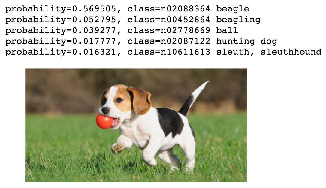
This fold contains examples for image classification. The goal of image classifcation is to identify the objects contained in images. The following example shows recognized object classes with corresponding probabilities using a pre-traind model.
- Basic usages
- How to prepare datasets
- A List of pre-trained models
- How to fine-tune a dataset with a pre-trained model
- How to train with multiple machines
- Frequently asked questions
Both python and R training programs are provided. Use train_*.py or
train_*.R to train a network on a particular dataset. For example:
-
train a multilayer perception on the mnist dataset
python train_mnist.py --network mlp
-
train a 110-layer resnet on the cifar10 dataset with batch size 128 and GPU 0 and 1
python train_cifar10.py --network resnet --num-layers 110 --batch-size 128 --gpus 0,1
There is a rich set of options, one can list them by passing --help. Some
commonly used options are listed as following:
| Argument | Comments |
|---|---|
network |
The network to train, which is defined in symbol/. Some networks may accept additional arguments, such as --num-layers is used to specify the number of layers in ResNet. |
data-train, data-val |
The data for training and validation. It can be either a filename or a directory. For the latter, all files in the directory will be used. But if --benchmark 1 is used, then there two arguments will be ignored. |
gpus |
The list of GPUs to use, such as 0 or 0,3,4,7. If an empty string '' is given, then we will use CPU. |
batch-size |
The batch size for SGD training. It specifies the number of examples used for each SGD iteration. If we use k GPUs, then each GPU will compute batch_size/k examples in each time. |
model |
The model name to save (and load). A model will be saved into two parts: model-symbol.json for the network definition and model-n.params for the parameters saved on epoch n. |
num-epochs |
The maximal number of epochs to train. |
load-epoch |
If given integer k, then resume the training starting from epoch k with the model saved at the end of epoch k-1. Note that the training starts from epoch 0, and the model saved at the end of this epoch will be model-0001.params. |
lr |
The initial learning rate, namely for epoch 0. |
lr-factor, lr-step-epochs |
Reduce the learning rate on give epochs. For example, --lr-factor .1 --lr-step-epochs 30,60 will reduce the learning rate by 0.1 on epoch 30, and then reduce it by 0.1 again on epoch 60. |
The recommended data format is
RecordIO, which
concatenates multiple examples into seekable binary files for better read
efficiency. We provide a tool im2rec.py located in tools/ to convert
individual images into .rec files.
For a simple tutorial, assume all images are stored as individual image files
such as .png or .jpg, and images belonging to the same class are placed in
the same directory. All these class directories are then in the same root
img_data directory. Our goal is to generate two files, mydata_train.rec for
training and mydata_val.rec for validation, and the former contains 95%
images.
We first prepare two .lst files, which consist of the labels and image paths
can be used for generating rec files.
python tools/im2rec.py --list True --recursive True --train-ratio 0.95 mydata img_dataThen we generate the .rec files. We resize the images such that the short edge
is at least 480px and save them with 95/100 quality. We also use 16 threads to
accelerate the packing.
python tools/im2rec.py --resize 480 --quality 95 --num-thread 16 mydata img_dataHints:
- SSD is much faster than HDD when dealing with a large number of small
files. (but HDD is good enough to read
recfiles).-
We can use a cloud storage instance to prepare the data. For example, AWS
i2.4xlargeprovides 4 x 800 GB SSDs. -
We can make a software RAID over multiple disks. For example, the following command create a RAID0 on 4 disks:
sudo mdadm --create --verbose /dev/md0 --level=stripe --raid-devices=4 \
  /dev/nvme0n1 /dev/nvme1n1 /dev/nvme2n1 /dev/nvme3n1
sudo mkfs /dev/md0
-
- Check
*.shscripts in thedata/folder for more examples - Use
im2rec.py --helpto see more options.
We provide multiple pre-trained models on various datasets. Use common/modelzone.py to download these models. These models can be used in any front-end language MXNet supports. For example, the tutorial shows how to classify an image with jupyter notebook.
It is first used by ImageNet challenge 2012, which contains about 1.2M images with 1000 classes. To test these models, one can use data/imagenet1k-val.sh to prepare the validation dataset and score.py to calculate the accuracy.
| Model | Top-1 | Top-5 |
|---|---|---|
imagenet1k-inception-bn |
0.7245 | 0.9079 |
imagenet1k-resnet-18 |
0.6858 | 0.8866 |
imagenet1k-resnet-34 |
0.7244 | 0.9097 |
imagenet1k-resnet-50 |
0.7527 | 0.9258 |
imagenet1k-resnet-101 |
0.7684 | 0.9327 |
imagenet1k-resnet-152 |
0.7653 | 0.9312 |
imagenet1k-resnext-50 |
0.7689 | 0.9332 |
imagenet1k-resnext-101 |
0.7828 | 0.9408 |
Note:
- our Resnet dose not need to specify the RGB mean due the data batch
normalization layer. While the inception models needs
--rgb-mean 123.68,116.779,103.939 - Resnet training logs are available at tornadomeet/ResNet
Single K80 GPU with batch size 32.
| Model | memory (MB) | images/sec |
|---|---|---|
imagenet1k-inception-bn |
548 | 152 |
imagenet1k-resnet-18 |
637 | 185 |
imagenet1k-resnet-34 |
678 | 172 |
imagenet1k-resnet-50 |
763 | 109 |
imagenet1k-resnet-101 |
835 | 78 |
imagenet1k-resnet-152 |
897 | 57 |
It is generated from the complete Imagenet dataset, namely fall11_whole.tar
from
http://www.image-net.org/download-images. In
addition, we removed classes which have less than 500 images, and then randomly
picked 50 images from each class as the validation set. As a result, this
dataset contains 11221 classes, with 11,797,630 images for training.
| Model | Top-1 |
|---|---|
imagenet11k-resnet-152 |
0.4157 |
This dataset combine the Imagenet 11K dataset with the Place 365 challenge dataset. The latter contains 365 classes with 8 millions images. It results in a dataset with around 20 million images.
| Model | Top-1 |
|---|---|
imagenet11k-place365ch-resnet-50 |
0.3112 |
imagenet11k-place365ch-resnet-152 |
0.3355 |
Fine-tune refers training with parameters partially intialized with pre-trained
model. One can use
fine-tune.py
to train another dataset with pre-trained models listed above. For example,
first run
data/caltech256.sh
to download and prepare the
Caltech-256 dataset,
then fine tune it with imagenet11k-resnet-152 by using 8 GPUs:
python fine-tune.py --pretrained-model imagenet11k-resnet-152 --gpus 0,1,2,3,4,5,6,7 \
    --data-train data/caltech256-train.rec --data-val data/caltech256-val.rec \
    --batch-size 128 --num-classes 256 --num-examples 15240
We obtained 87.3% top-1 validation accuracy, and the training log is available here. See the python notebook for more explanations.
The simplest way for distributing training is that both programs and data are
placed on the a shared filesystem such as
NFS and
AWS EFS, and there is one machine, we call it the
root machine, can ssh to all others. Assume we save the hostnames (or IPs) of
all machines will be used for training (might include the root machine) into a
file named hosts. The outputs of cat hosts may be
172.30.0.172
172.30.0.171
Now we can run the previous cifar10 training on two machines:
../../tools/launch.py -n 2 -H hosts \
    python train_cifar10.py --network resnet --num-layers 110 --batch-size 128 --gpus 0,1 \
    --kv-store dist_device_sync
It differs the previous command in two aspects. First, we use launch.py to
start the program, which creates two workers (given by -n) on the two machines
specified in hosts . Second, we change the --kv-store from the default
device, which means try to use GPU P2P, to dist_device_sync. The latter uses
distributed synchronized communication.
For more usages:
- One can use benchmark.py to run distributed benchmarks (also for multiple GPUs with single machine)
- A how-to tutorial with more explanation.
- A blog about setuping up a GPU cluster on AWS with cloud formation.
To run benchmark on imagenet networks, use --benchmark 1 as the argument to train_imagenet.py, An example is shown below:
python train_imagenet.py --benchmark 1 --gpus 0,1 --network inception-v3 --batch-size 64 \
  --image-shape 3,299,299 --num-epochs 1 --kv-store device
When running in benchmark mode, the script generates synthetic data of the given data shape and batch size.
The benchmark.py can be used to run a series of benchmarks against different image networks on a given set of workers and takes the following arguments:
--worker_file: file that contains a list of worker hostnames or list of worker ip addresses that have passwordless ssh enabled.--worker_count: number of workers to run benchmark on.--gpu_count: number of gpus on each worker to use.--networks: one or more networks in the format network_name:batch_size:image_size.
The benchmark.py script runs benchmarks on variable number of gpus upto gpu_count starting from 1 gpu doubling the number of gpus in each run using kv-store=device and after that running on variable number of nodes on all gpus starting with 1 node upto worker_count doubling the number of nodes used in each run using kv-store=dist_sync_device.
An example to run the benchmark script is shown below with 8 workers and 16 gpus on each worker:
python benchmark.py --worker_file /opt/deeplearning/workers --worker_count 8 \
  --gpu_count 16 --networks 'inception-v3:32:299'
- Hardware: 16x AWS P2.16xlarge with 256 GPUs in total.
- Software: AWS Deep Learning AMI with CUDA 7.5 and CUDNN 5.1 installed
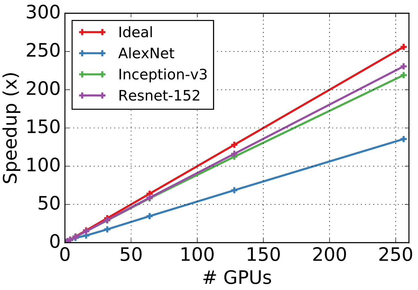
We fixed the batch size per GPU and then increase the number of
GPUs. Synchronized SGD is used, namely --kv-store dist_device_sync. The
following three CNNs (located in symbol/) are used
alexnet |
inception-v3 |
resnet-152 |
|
|---|---|---|---|
| batch per GPU | 512 | 32 | 32 |
| model size (MB) | 203 | 95 | 240 |
Number of images proccessed per second is shown in the following table:
| #GPUs | alexnet |
inception-v3 |
resnet-152 |
|---|---|---|---|
| 1 | 457.07 | 30.4 | 20.08 |
| 2 | 870.43 | 59.61 | 38.76 |
| 4 | 1514.8 | 117.9 | 77.01 |
| 8 | 2852.5 | 233.39 | 153.07 |
| 16 | 4244.18 | 447.61 | 298.03 |
| 32 | 7945.57 | 882.57 | 595.53 |
| 64 | 15840.52 | 1761.24 | 1179.86 |
| 128 | 31334.88 | 3416.2 | 2333.47 |
| 256 | 61938.36 | 6660.98 | 4630.42 |
The following figure shows the speedup against a single GPU compared to the ideal scalability.
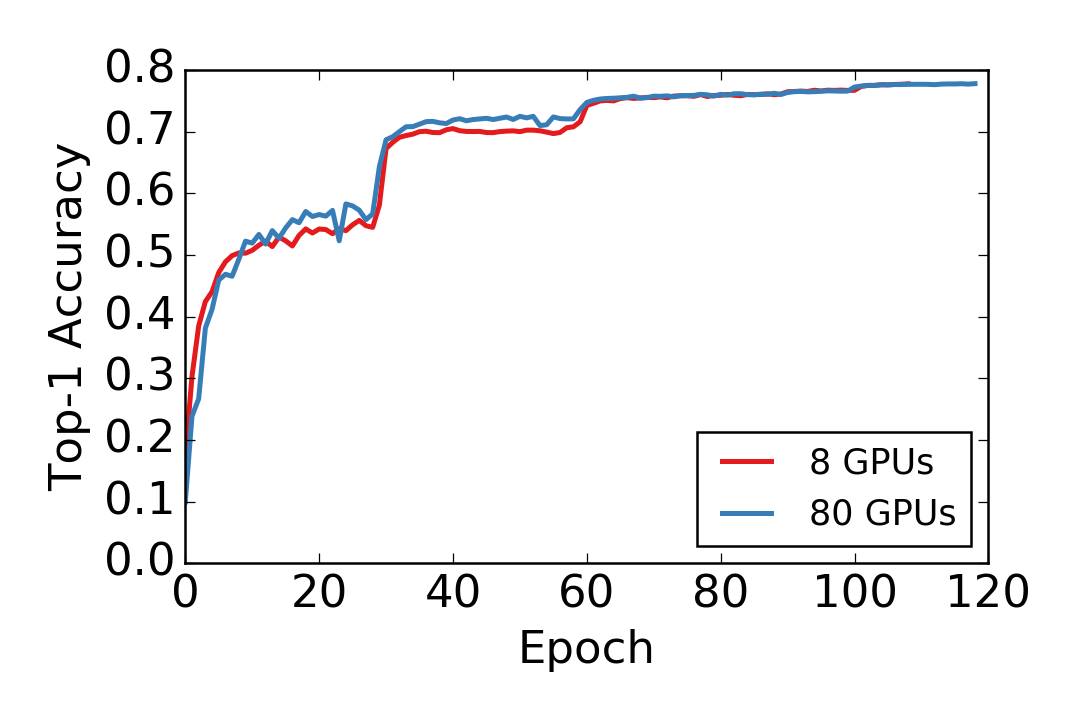
We show the convergence of training ResNet-152 on Imagenet 1K. The single machine with 8 GPUs results are from Wei Wu. We then trained the model using 10 machines, each machine has 8 GPUs, with the same hyper-parameters, except for we changed the total batch size from 8*32 to 80*32 and the initial learning rate to 0.5 instead of 0.1. The validationn accuracy versus data epoch is shown as following. Both models have almost identical convergence rate.
It is often straightforward to achieve a reasonable validation accuracy, but sometimes matching the state-of-the-art numbers reported in the papers is extremely hard. Here we list some aspects you may check to improve the validation accuracy:
- Add more data argumentations, which often reduces the gap between training accuracy and validation accuracy. You may reduce the data argumentation close to end.
- Increase the learning rate and keep large learning rate for a long time. For
example, in CIFAR10 we keep
lr=0.1for 200 epochs and then reduce to 0.01. - Do not use too large batch size, especially for batch size >> number of classes.
First check the workload is not too small (e.g. LeNet on MNIST) and also batch size is reasonable large. The performance bottleneck often happens in three aspects:
- Reading data. Use the
--test-io 1flag to check how many images can be pre-processed per second- Increase
--data-nthreads(default is 4) to use more threads for data augmentation can help. - Data preprocessing is done by
opencv. If opencv is compiled from source codes, check if it is configured correctly. - Use
--benchmark 1to use randomly generated data rather than real data.
- Increase
- CPU performance. Check MKL DNN is used, namely set
USE_MKL2017 = 1andUSE_MKL2017_EXPERIMENTAL = 1to compile - Single GPU performace
- Check the recent CUDNN is used
- Check the environment variable
MXNET_CUDNN_AUTOTUNE_DEFAULTis set to 1. You can do it byexport MXNET_CUDNN_AUTOTUNE_DEFAULT=1; python train_.... Note that it is already enabled in default bycommon/find_mxnet.py. Enabling it results 15% speedup in average, but it may cause problems for RNN and bucketing, and also slow down the starting.
- Multiple GPUs and multi-machine performance. The bottleneck is often on the
communication bandwidth, you can use
tools/bandwidth
to find the communication cost per batch. A ideal situation is the cost is
less than the time to compute a batch. We can
- Explore different
--kv-storeoptions to reduce the cost - Increase the batch size to improve the computation and communication ratio.
- Explore different
An over sized batch size may result in out of GPU memory. The common error
message is cudaMalloc failed: out of memory. Now we can
- Reduce the batch size
- Set the environment variable
MXNET_BACKWARD_DO_MIRRORto 1. It trades off computation for memory consumption. For example, with batch size 64, inception-v3 uses 10G memory and trains 30 image/sec on a single K80 GPU. When mirroring is enabled, with 10G GPU memory consumption, we can run inception-v3 using batch size 128. The cost is that the speed reduces to 27 images/sec.
- Nov 9, 2015: major refactor.
- Organize files into sub-directories
- Add Resnet, pretrained models, and fine-tune scripts.
- Update documents.
- Move
../cpp/image-classificationinto./predict-cpp/
- Oct 15, 2016: add R examples
- Nov 19, 2015: major refactor.
- Various networks (Alex/VGG/Inception) on multiple dataset (MNIST/Cifar10/Imagenet)
- Distributed training


