README.md

ActuaryUtilities

Quickstart

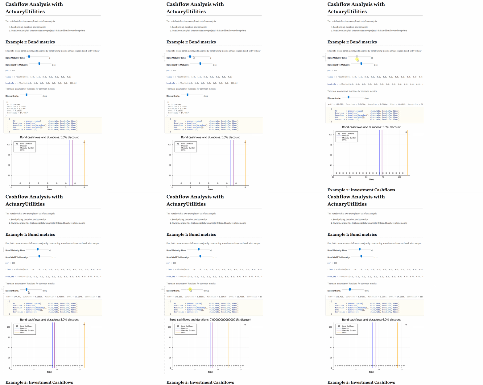
cfs = [5, 5, 105]
times    = [1, 2, 3]

discount_rate = 0.03

present_value(discount_rate, cfs, times)           # 105.65
duration(Macaulay(), discount_rate, cfs, times)    #   2.86
duration(discount_rate, cfs, times)                #   2.78
convexity(discount_rate, cfs, times)               #  10.62

Features

A collection of common functions/manipulations used in Actuarial Calculations.

Financial Maths

• duration:
  • Calculate the Macaulay, Modified, or DV01 durations for a set of cashflows
  • Calculate the KeyRate(time) (a.k.a. KeyRateZero)duration or KeyRatePar(time) duration
• convexity for price sensitivity
• Flexible interest rate models via the FinanceModels.jl package.
• internal_rate_of_return or irr to calculate the IRR given cashflows (including at timepoints like Excel's XIRR)
• breakeven to calculate the breakeven time for a set of cashflows
• accum_offset to calculate accumulations like survivorship from a mortality vector
• spread will calculate the spread needed between two yield curves to equate a set of cashflows

Risk Measures

• Calculate risk measures for a given vector of risks:
  • CTE for the Conditional Tail Expectation
  • VaR for the percentile/Value at Risk
  • WangTransform for the Wang Transformation
  • ProportionalHazard for proportional hazards
  • DualPower for dual power measure

Insurance mechanics

• duration:
  • Calculate the duration given an issue date and date (a.k.a. policy duration)

Typed Rates

• functions which return a rate/yield will return a FinanceCore.Rate object. E.g. irr(cashflows) will return a Rate(0.05,Periodic(1)) instead of just a 0.05 (float64) to convey the compounding frequency. This is compatible across the JuliaActuary ecosystem and can be used anywhere you would otherwise use a simple floating point rate.

A couple of other notes:

• rate(...) will return the scalar rate value from a Rate struct:

julia> r = Rate(0.05,Periodic(1));

julia> rate(r) 
0.05

• You can still pass a simple floating point rate to various methods. E.g. these two are the same (the default compounding convention is periodic once per period):

discount(0.05,cashflows)

r = Rate(0.05,Periodic(1));
discount(r,cashflows)

• convert between rates with:

r = Rate(0.05,Periodic(1));

convert(Periodic(2),  r)   # convert to compounded twice per timestep
convert(Continuous(2),r)   # convert to compounded twice per timestep

For more on Rates, see FinanceCore.jl. FinanceModels.jl also provides a rich and flexible set of yield models to use.

Documentation

Full documentation is available here.

Examples

Interactive, basic cashflow analysis

See JuliaActuary.org for instructions on running this example.

Useful tips

Functions often use a mix of interest_rates, cashflows, and timepoints. When calling functions, the general order of the arguments is 1) interest rates, 2) cashflows, and 3) timepoints.