calculations_basic_workflow.Rmd

# Calculations: basic workflow {#calcs-basic} 

The purpose of Chapter \@ref(calcs-basic) is to introduce you to the basic workflow for calculating OHI scores. This is a 2-hour hands-on training: you will be following along on your own computer and working with a copy of the demonstration repository that is used throughout this chapter.

## Overview

Calculating scores with the OHI Toolbox requires a tailored repository operating with the OHI `R` package `ohicore`. The tailored repo has information specific to your assessment — most importantly the data and goal models — and `ohicore` will combine these with core operations to calculate OHI scores. You will always start with a tailored repository that has data and models extracted from the most recent Global OHI assessment.

This training will introduce the basic workflow for calculating scores. There are many ways to build from the 'out-of-the-box' tailored repo you have instead of starting an assessment from scratch. For example, you may want to just change underlying data sources within the models, or completely change the models which also requires new data layers and data sources. 

**We will repeat the basic workflow four times, each time adding complexity. We will calculate scores with:**

1. 'out of the box' data and models extracted from a recent global assessment
1. tailored data (with 'out of the box' models)
    - explore Configure Toolbox section
    - explore `functions.R`
1. tailored models (with 'out of the box' data layers)
1. tailored data and models (adding a new data layer / model variable)

<br>

The workflow depends on the `calculate_scores.Rmd` file found the scenario folder of any tailored repo. We'll also dive deeper into the code itself, focusing particularly on developing goal models in `functions.R`. 
**Note:** *earlier Toolbox versions have `calculate_scores.R` which calls `configure_toolbox.R`. Now, `calculate_scores.Rmd` has a section named "Configure Toolbox", which has the equivalent code so it is possible to follow along with this tutorial even if your repository does not have the `.Rmd`.* 

This is a lot to cover in a 2-hour training, and the purpose is to give you big take home messages and experience for what you need to begin calculating scores. But the Toolbox has a lot of moving parts, and we cannot cover all of it here. There are a lot of details and other operations that we won't get into here and that will be coming in future tutorials (including tailoring pressures & resilience, and how to change subgoals). 


### Prerequisites

Before the training, please make sure you have done the following: 

1. Have up-to-date versions of `R` and RStudio and have RStudio configured with Git/GitHub <!--- TODO (Chapter \@ref(datascience))--->
    - https://cloud.r-project.org
    - http://www.rstudio.com/download 
    - http://happygitwithr.com/rstudio-git-github.html 
1. Fork the **toolbox-demo** repository into your own GitHub account by going to https://github.com/OHI-Science/toolbox-demo, clicking "Fork" in the upper right corner, and selecting your account
1. Clone the **toolbox-demo** repo from your GitHub account into RStudio into a folder called "github" in your home directory (filepath "~/github")
1. Get comfortable: be set up with two screens if possible. You will be following along in RStudio on your own computer while also watching an instructor's screen or following this tutorial.

----

## Review the Toolbox file ecosystem

Let's quickly review some of the files you have in the **toolbox-demo** repo that we saw in Chapter \@ref(toolbox-ecosystem). Remember that the ecosystem structure of any tailored repo is the same, so as you learn to navigate through and calculate scores in this repo you are also learning how to navigate through and calculate scores in any other OHI assessment repository — yours or anyone else's.

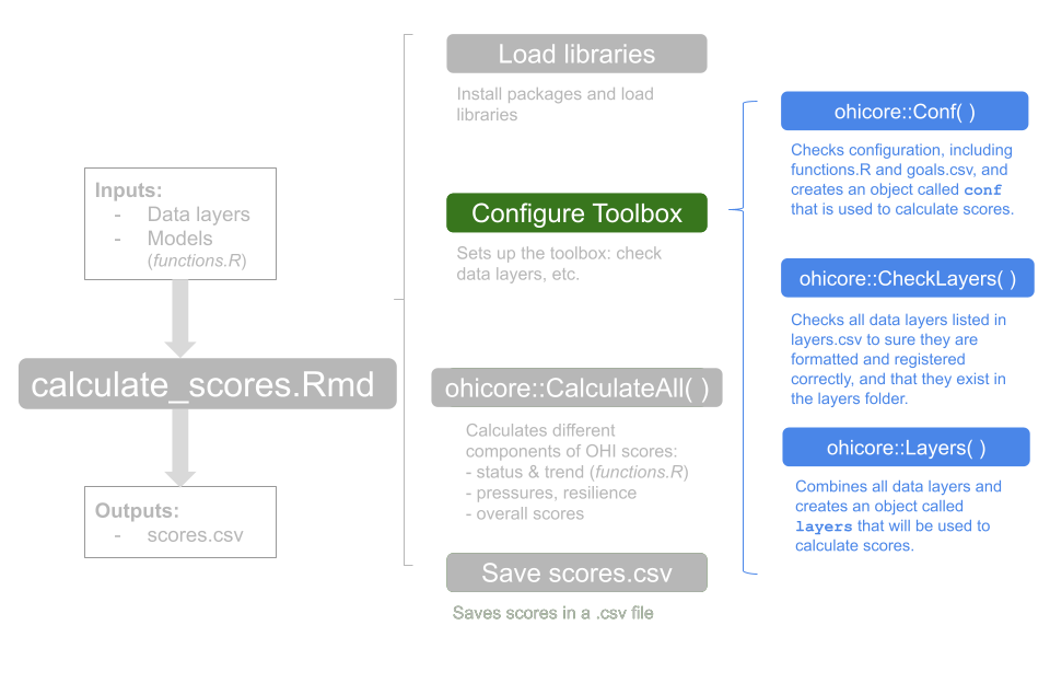
This figure highlights the files we will focus on in this tutorial (others are grayed out). 

![](https://docs.google.com/drawings/d/e/2PACX-1vRDZg3ubeNFMEJ2eBtoLb0YJKgUHTOhZEbE8DMHivSLputNULN2guzL0p_LWSDC2O8wiQLpIX589e6Z/pub?w=960&h=600)

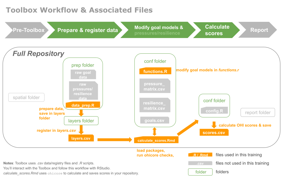
In our **toolbox-demo** repo, here are a few additional things to mention: 

- our scenario folder is called `region2017`
- goal models are `R` functions all stored in `conf/functions.R`
- regions are listed (with area) in `spatial/regions_list.csv`. We have 8 here.
- <!---TODO:: Learn more about the `ohicore` package: [ohi-science.org/ohicore](http://ohi-science.org/ohicore)---> 


## Calculate with 'out-of-the-box' data and models

The first time we go through the basic workflow will be with 'out-of-the-box' data and models from the global assessment. 

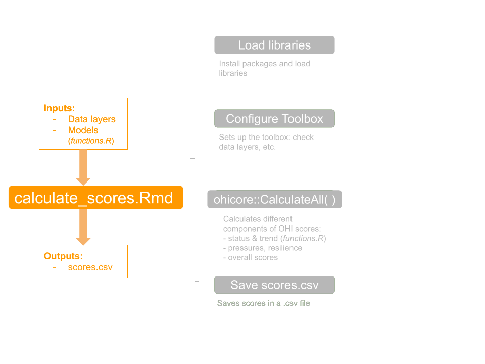
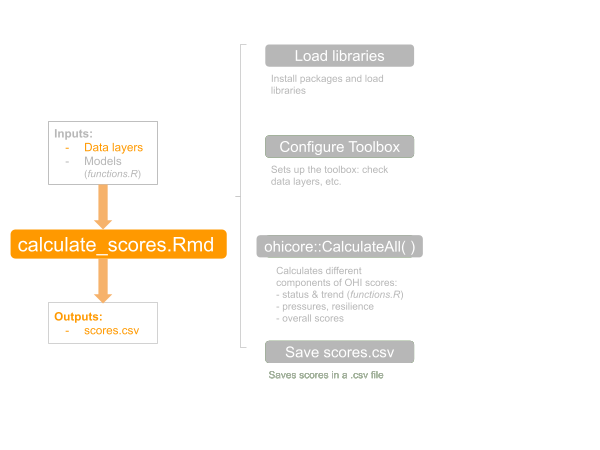
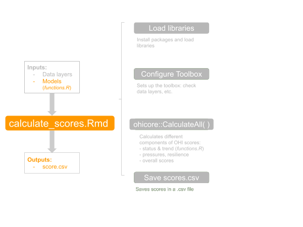
`calculate_scores.Rmd` is the file that you'll use a lot — mostly to run piece-by-piece as you develop your models. It takes inputs (data and models) from your repository and uses the OHI R package `ohicore` to compute OHI scores. It has several components which we will explore in turn in the rest of  the tutorial. 

![](https://docs.google.com/drawings/d/1OhA7p5-dmrk6dGeP_gWEXFD2pI1ik8KhUYNUSLUVgd4/pub?w=960&h=720)

<br>

`calculate_scores.Rmd` will load the libraries you need and `ohicore` will check your book-keeping and configuration, and calculate OHI scores. **Ultimately, it will save the scores for each goal and dimension in `scores.csv`.** The 'dimensions' of OHI goal scores are Status, Trend, Pressures, Resilience, Likely Future State, and overall goal Score. Dimensions are calculated for each goal in a specific order, as we will see below. `calculate_scores.Rmd` will combine information from your tailored repository and calculate scores with OHI core functions from `ohicore`. 

Open `region2017/calculate_scores.Rmd` and let's have a look at its operations. We will then run it line-by-line.

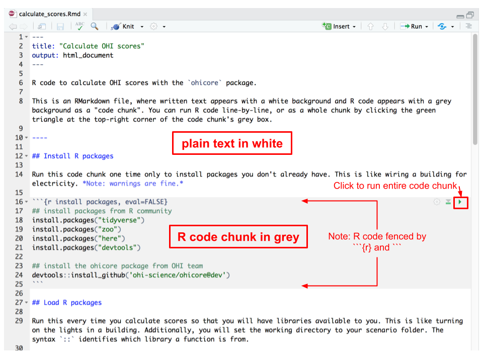
`calculate_scores.Rmd` is an [RMarkdown](https://rmarkdown.rstudio.com/) file, which combines simply formatted text and R code and is really amazing for communication, including our OHI websites (see a 1-minute video [here](https://vimeo.com/178485416)). For now, we will focus on the .Rmd file within the RStudio pane, and see that written text appears with a white background and R code appears with a grey background as a "code chunk". You can run R code line-by-line, or as a whole chunk by clicking the green triangle at the top-right corner of the code chunk's grey box. 

![](https://docs.google.com/drawings/d/e/2PACX-1vQ3JLCA6A1iXLMsPBMLTJJSsUGfD6mEKOEROUALlcSH6f-VMLOgPL0Kwe4S4YHackdHPXvSFPIQcBL7/pub?w=960&h=720)

<br>

Each of the following steps is its own section and code chunk within `calculate_scores.Rmd`.

### Install packages, including `ohicore`

**Note**: *Previous versions of the Toolbox had `install_ohicore.r` as a separate file, but the effect is the same.*

OHI requires packages created by others in the R community as well as one we developed ourselves. This is something that only needs to be done one time. I think of it as wiring a building for electricity: once it's done, it's done. Let's run these line-by-line if you don't have them installed already.

`ohicore` is an R package developed by the OHI team that has all the essential core functions and supporting packages you will use to develop your assessment and calculate scores.

```{r install packages, eval=FALSE}
## install packages from R community
install.packages("tidyverse")
install.packages("zoo")
install.packages("here")
install.packages("devtools")

## install the ohicore package from OHI team
devtools::install_github('ohi-science/ohicore@dev')
```

### Load R packages

Next, you will load each R package as a library from the `toolbox-training` repository whenever you work on your assessment to gain access to all those functions and packages. That is like turning on the lights when you need to use them; you need to do this every time you open your assessment repository. 

We will also set the working directory, because the `ohicore` package expects you to be inside your scenario folder (this will be improved further another time). We will use the new `here` package, which will identify the full filepath on your computer and will make collaborating easier between us.

```{r setup, eval=FALSE}
## load package libraries
library(tidyverse)
library(stringr)
library(zoo)
library(here)
library(ohicore)

## set the working directory to a filepath we all have
setwd(here::here('region2017'))
```

### Configure the Toolbox

Next, we will configure the toolbox from within `calculate_scores.Rmd`. Let's run the whole code chunk by clicking the green arrow at the top-right. 

There is output printed to the console that lists all of the layers registered, and ends with any warning messages about the layers themselves. We will explore what is happening here and how to interpret these warning messages further on; for now, let's move on since we have not encountered an error. 

```{r configure_toolbox, eval=FALSE}
conf <- ohicore::Conf('conf')

## check that scenario layers files in the \layers folder match layers.csv registration. Layers files are not modified.
ohicore::CheckLayers('layers.csv', 'layers', flds_id=conf$config$layers_id_fields)

## load scenario layers for ohicore to access. Layers files are not modified.
layers <- ohicore::Layers('layers.csv', 'layers')

## select corresponding data year to use for pressures and resilience
scenario_years <- 2016
layers$data$scenario_year <- scenario_years

#   cc_acid
#   cc_slr
# ...
#   tr_travelwarnings
# Warning messages:
# 1: In ohicore::CheckLayers("layers.csv", "layers", flds_id = conf$config$layers_id_fields) :
#   Unused fields...
#     ico_spp_iucn_status: iucn_sid
# 2: In ohicore::CheckLayers("layers.csv", "layers", flds_id = conf$config$layers_id_fields) :
#   Rows duplicated...
#     ico_spp_iucn_status: 816

```

### Calculate Scores

Now let's continue with the next code chunk in `calculate_scores.Rmd`, which first **runs `CalculateAll()`**. Notice too that we are saving the output to a variable called `scores`. Instead of running the whole code chunk here, let's just run this single line.

> Note: the prefix `ohicore::` is a way to be explicit that the `CalculateAll()` is part of the `ohicore` package.

```{r CalculateAll, eval=FALSE}
## calculate scenario scores
scores <-  ohicore::CalculateAll(conf, layers)
```

#### Output: Status and Trend 

`CalculateAll()` first calculates the Status and Trend for every goal and subgoal. These models are in your tailored repository's `functions.R` (we will explore `functions.R` below). You can choose to add messages to print during calculation like is shown below for Mariculture (MAR).

```{r CalculateAll_output_status, eval=FALSE}
# Running Setup()...
# Calculating Status and Trend for each region for FIS...
# Calculating Status and Trend for each region for MAR...
# 95th percentile for MAR ref pt is: 0.0758396517531756
# ... 
```

#### Output: Pressures and Resilience 

Next, we see output as `CalculateAll()` calculates Pressures and Resilience based on the pressures and resilience matrix tables in your tailored repository. For each, `ohicore` lists the subcategories that will be calculated, and identifies any mismatches between data layers identified but not used or missing. We will learn more about the pressures and resilience matrices in a different Chapter. <!---TODO: need to develop the pressures/resilience chapter and link---> 

```{r CalculateAll_output_pressures, eval=FALSE}
# Calculating Pressures for each region...

# There are 6 pressures subcategories: pollution, alien_species, habitat_destruction, fishing_pressure, climate_change, social
# These goal-elements are in the weighting data layers, but not included in the pressure_matrix.csv:
# LIV-aqf
# These goal-elements are in the pressure_matrix.csv, but not included in the weighting data layers:
# CP-coral, CP-mangrove, CP-saltmarsh, CS-mangrove, CS-saltmarsh, HAB-coral, HAB-mangrove, HAB-saltmarsh, HAB-seagrass, LIV-ph, LIV-tran, CP-seaice_shoreline, HAB-seaice_edge, ECO-wte, LIV-wte, LIV-sb


# Calculating Resilience for each region...

# There are 7 Resilience subcategories: ecological, alien_species, goal, fishing_pressure, habitat_destruction, pollution, social
# These goal-elements are in the resilience_matrix.csv, but not included in the weighting data layers:
# CP-coral, CP-saltmarsh, CS-saltmarsh, HAB-coral, HAB-saltmarsh, HAB-seagrass, CP-mangrove, CS-mangrove, HAB-mangrove, HAB-seaice_edge, CP-seaice_shoreline
```

#### Output: Combine Dimensions

Finally, we see output as `CalculateAll()` combines the dimensions above in several ways. It calculates the Goal Scores and Likely Future State for each goal and subgoal. Then, it calculates 'supragoals', which are goals that have subgoals, for example Food Provision (FP), which has the subgoals FIS (Wild-caught Fisheries) and Mariculture (MAR). Finally, it calculates the overall Index score for the entire Assessment Area using an area-weighted average. 

```{r CalculateAll_output_etc, eval=FALSE}
# ...
# Calculating Goal Score and Likely Future for each region for FIS...
# Calculating Goal Score and Likely Future for each region for MAR...
# ...
# Calculating post-Index function for each region for FP...
# Calculating post-Index function for each region for LE...
# Calculating Index score for each region for supragoals using goal weights...
# Calculating Likely Future State for each region for supragoals using goal weights...
# Calculating scores for ASSESSMENT AREA (region_id=0) by area weighting...
# Calculating FinalizeScores function...
```

#### Output: Warning Messages

Following all the calculations are the warning messages, which are due to operations within `functions.R`, which you will be able to fix as you tailor your goal models. These warning messages are due to using goal models from the global assessment with just a subset of data from the global assessment we have extracted here for the **toolbox-demo** repository.

```{r CalculateAll_output_warnings, eval=FALSE}
# Warning messages:
# 1: In left_join_impl(x, y, by$x, by$y, suffix$x, suffix$y) :
#   joining factors with different levels, coercing to character vector
# ...
# 8: In max(d$x, na.rm = T) :
#   no non-missing arguments to max; returning -Inf
```

### Save scores variable as `scores.csv`

Finally, we will save the output from `CalculateAll()`, a variable called `scores`, as a comma-separated-value file called `scores.csv`. We will do this by running the second line of code in this code chunk.

```{r write_scores, eval=FALSE}
## save scores as scores.csv
readr::write_csv(scores, 'scores.csv', na='')
```

We can inspect it and see that it is a long-formatted file with four columns for the goal, dimension, numeric region identifier, and score. 

|goal |dimension | region_id| score|
|:----|:---------|---------:|-----:|
|AO   |future    |         0| 92.85|
|AO   |future    |         1| 92.85|
|AO   |future    |         2| 92.85|
|...  |...       |       ...|  ... |
|AO   |pressures |         1| 37.75|
|AO   |pressures |         2| 37.75|
|...  |...       |       ...|  ... |

We have 8 regions in the **toolbox-demo** repo. An additional region 0 is the area-weighted combination of all regions.

> Note: each region in your assessment will have a numeric region identifer, called a `region_id` or `rgn_id` for short. You can see a list of all regions and corresponding identifiers in [toolbox-demo/region2017/spatial/regions_list.csv](https://github.com/OHI-Science/toolbox-demo/blob/master/region2017/spatial/regions_list.csv)


### Error messages

Hopefully this first time through `calculate_scores.Rmd` you did not encounter error messages, but you definitely will as you move ahead. Error messages are often due to typos or miscommunications between what you tell `R` versus what it expects. You will encounter error messages due to `R` itself, and due to `ohicore`. Error messages often have human-friendly messages to alert you to what went wrong, and we are continually improving error messages you'll encounter when you use `ohicore` so you can try to solve them more easily. Some commonly occurring errors and how to fix them can be found in the Troubleshooting section of the manual. Copy-pasting error messages into Google is also one of the best places to start. 

### Create figures

Two common plots to represent scores are flower plots and maps. We will walk through an example of the flower plot code here. **Note**: you'll see that we are sourcing code from another OHI repository, where this code was developed. After we finish testing it, we will add it as a function to `ohicore` and then you will not need to source it anymore. 

```{r plot, eval=FALSE}
## source script (to be incorporated into ohicore)
source('https://raw.githubusercontent.com/OHI-Science/arc/master/circle2016/plot_flower_local.R')

PlotFlower(assessment_name = "Toolbox Demo",
           dir_fig_save    = "reports/figures")
```

The default arguments is to create a flowerplot for every region and region 0, although you can modify this. When we run this code now you will see that the figures were in fact recreated (the timestamps for the figures in the File pane of RStudio have updated) but are not different from the previous ones so they do not show up in the Git window.

### Recap of first `calculate_scores.Rmd` run

We have just successfully run through the basic workflow to calculate OHI scores. It first loads necessary packages, configures data and models, and then it calculates all the components of OHI scores (status, trend, pressures, resilience, overall scores), and finally it saves the new OHI `scores` object in a .csv file.

We will build on this basic workflow, by exploring the operations above in more detail, and by updating the data, models, and configurations within the **toolbox-demo** repository. 

![](https://docs.google.com/drawings/d/1OhA7p5-dmrk6dGeP_gWEXFD2pI1ik8KhUYNUSLUVgd4/pub?w=960&h=720)


## Calculate with tailored data

Now let's run through this basic workflow a second time, building on what we've learned. 

Here, we will focus on one of the layers for the Artisanal Fishing Opportunity (AO) goal. We will prepare local data that will substitute global data for the data layer `ao_access` and recalculate scores without modifying the goal model itself.

![](https://docs.google.com/drawings/d/1kRwkY_vqAXh-nACsS39ZHEVYW_zsGSFiKs_-5W6swBs/pub?h=450)

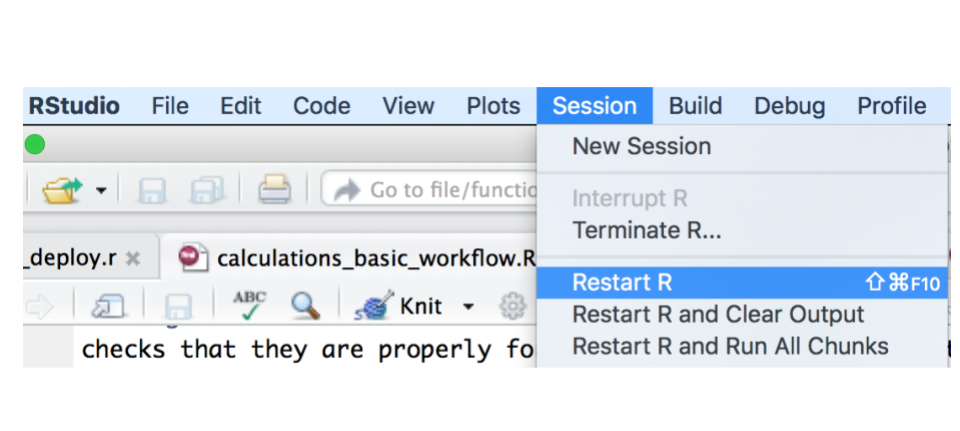
It's a good idea to go to RStudio's Session menu and select Restart `R` to make sure you have a clean working directory.

![](https://docs.google.com/drawings/d/1FmN6httmUUOcz1a1-2XjXxOnVWsZ8t68mVVGFSg7F1E/pub?w=960&h=432)

### Prepare and save our data layer

While Chapter \@ref(prep-data) shows in detail how to prepare data layers, save them in the "layers" folder, and register them in `layers.csv` and `scenario_data_years.csv` so the Toolbox knows where to find them, we have prepared a shorter example with AO for our purposes here. 

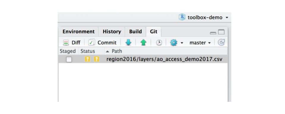
Open `toolbox-demo/prep/AO/access_prep.R` and source it after reading it through. The result will be a new data file called "ao_access_demo2017.csv" saved to the "layers" folder, and you should see that there is a new file saved in your Git window. 

![](https://docs.google.com/drawings/d/1ED1Xk2WELXm5y8edbWr_s9kjvm3TpSK80Via05e9Cog/pub?w=960&h=384)

### Register in `layers.csv`

Now that we have prepared and saved our data layer, we'll register it in `layers.csv`. `layers.csv`is a registry that will direct `ohicore` to appropriate data layers, and has information about each data layer — which goal it is used for, filename, column names, etc. For further detail see Chapter \@ref(prep-data).

There is a data layer for `ao_access` that is already registered in `layers.csv`, but it is currently created from a file called "ao_access_gl2017.csv". We will update this so the data layer is created from our new demo file ("ao_access_demo2017.csv"); this happens in the "filename" column of `layers.csv`. 

Open `region2017/layers.csv` in a spreadsheet software (i.e. Microsoft Excel or Open Office). Next, find `ao_access` in the "layer" column. Where it says "ao_access_gl2017.csv", update this to say "ao_access_demo2017.csv" — the new data layer you just saved. Save this and close Excel. 

> IMPORTANT! Be sure to close Excel after you have made these edits. On a PC, having `layers.csv` open in Excel will prohibit it from being accessed from R, and the Toolbox needs access to calculate scores!

### Register in `scenario_data_years.csv`

Next let's go to `region2017/conf/scenario_data_years.csv`. We can open this in RStudio: when you click on its name in the Files pane, select "View File". 


`scenario_data_years.csv` is a registry to organize year information for each layer, and helps set you up from the very beginning to be able to calculate repeated assessments. When you calculate OHI scores, you will be explicit about the year your completed assessment represents, and we call this the `scenario_year`. `data_year` is the most recent years available for that data layer.

Let's look at the `ao_access` layer. It turns out that the same `data_year`, 2013, is used for all `scenario_years` 2008:2017. This means that this data source has not been updated through time so the trends that are calculated will be flat. We can double-check our "ao_access_demo2017.csv" file to see that 2013 is the most recent data that we have. This means that our data layer is already registered here in `scenario_data_years.csv` and we do not need to make any changes. 

Depending on your local data, registering in `scenario_data_years.csv` may be more like confirming the information that is already registered. Should you delete some of those previous years? Well, the Trend calculations require at least 5 years of data or the Toolbox will give errors. You can delete some of the earliest years to remove some clutter (left over from the global assessment), definitely rerun `calculate_scores.Rmd` afterwards to make sure that there are no unexpected changes to `scores.csv`

(As a side note, this would be a good data layer to substitute if you had better local information through time.) 

### Rerun `calculate_scores.Rmd` 

Now, let's rerun `calculate_scores.Rmd`. `ohicore` will now use your tailored data when it creates the "ao_access" layer because you've registered it in `layers.csv` and `scenario_data_years.csv` and the file is available in the layers folder. 

### Check our work, plot, and sync

Whenever there are changes made to your files (additions, deletions, and modifications), you will be notified in the Git window, since Git is tracking the files in this repo. This is a good place to confirm you have did the things you set out to do, and you can also see if you errantly did anything you didn't mean to.

So here, you added a new data layer and after calculating scores you expect to see changes to AO scores in `score.csv`. `layers.csv` will also change because `ohicore` will update fields in this file as it runs through its checks. But we don't expect any other files to change at this point, so let's make sure that's true. 

Now let's recreate the flower plots with our updated goal model. You'll see those .png's show up in the Git tab as well. Although we can't inspect the differences between the figures through RStudio here, we will be able to see them on GitHub.com. 

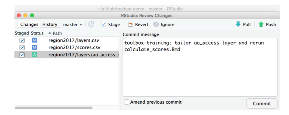
Now is a good time to commit this work and sync to GitHub. That way, the work we've done is committed together and we will have a clean slate (from a Git sense) moving forward. I'll use the commit message "toolbox-training: tailor ao_access layer and rerun calculate_scores.Rmd"

![](https://docs.google.com/drawings/d/1jwYB9w-O0Doae0KnoQjca_n4eY7D0E1NcW-VilIN_24/pub?w=960&h=384)

Now, we can inspect on GitHub.com: 

![](https://docs.google.com/drawings/d/e/2PACX-1vR_YSbMT4oizo7C4k9eKlV1fIGoaOG_ORpywd7ma8a36-0C-DiRl0qsGPY_qr8F8HlWgYCKQXsnu5Ru/pub?w=960&h=240)


### Recap of second `calculate_scores.Rmd` run

One way to tailor your assessment is to substitute data for an existing data layer. We have just run through the basic workflow a second time. This time we successfully: 

- substituted the global OHI data layer `ao_access` with new data, which includes saving it in `layers` folder, registering it in `layers.csv` and `scenario_data_years.csv`, and 
- reran `calculate_scores.Rmd` without modifying the goal model itself
- checked `scores.csv` changes in the Git tab to make sure all changes were expected 

## Explore Configure Toolbox

So now let's take a closer look at the Configure Toolbox section, the first code chunk following library install and loading in `calculate_scores.Rmd`. 

![](https://docs.google.com/drawings/d/e/2PACX-1vRfoNsoljXz9fjD4iitj982SGhBu_tof-yeCLVJTo4UTPBeKzNAXl0jP84Pjb_cpLFx-LUA9LfsMkeT/pub?w=960&h=624)

This code chunk combines everything required to calculate OHI scores and checks that they are properly formatted and available, and will minimize potential errors later on. It makes sure that your data and goal models are ready to be used to calculate scores. 


**Important: Any time you make a change to a data layer or a goal model and want to recalculate scores, you will need to re-run the Configure Toolbox code chunk to have `ohicore` operate on the most up-to-date information**. You can click the green triangle at the top right corner of the grey code chunk to run all the lines at the same time. We'll walk through line-by-line now.

### `ohicore::Conf()`

The `Conf()` function from `ohicore` (represented in code with the `ohicore::Conf()` syntax prepares for the next steps of running the Toolbox, and calls forth everything you need to calculate scores: 

- goal models
- other OHI parameters that determines how OHI scores are calculated 


```{r Conf(), eval=FALSE}
## load scenario configuration
conf <- ohicore::Conf('conf')
```

This function provides no output in the console, but does save a `conf` object that you can see in the Environment tab of RStudio.

### `ohicore::CheckLayers()`

The `CheckLayers()` function from `ohicore` checks that data layers are properly formatted and registered (e.g., that each data layer in `layers.csv` exists in the layers folder), and returns a list of all of the layers that are registered in the console. Check to make sure ours is there. This is a gate-keeping step by to make sure the data layers you've entered are in the right format and can be read by `ohicore` properly. 

```{r CheckLayers(), eval=FALSE}
## check that layers in the layers folder match layers.csv registration. 
ohicore::CheckLayers('layers.csv', 'layers', flds_id=conf$config$layers_id_fields)
```

In the R console, you will see a list of all data layers registered, and there will be additional warning information about specific layers at the end. You should not get an error at this point, but if you do, the list will stop printing where the error occurs, which will help you troubleshoot.

#### Warning messages 

Warning messages alert you to problems with specific layers: this is showing that there are unused fields and duplicate rows. These warning messages are not a problem now (they are a byproduct of extracting this repo based on global assessments; you'll be changing this layer anyways). 

```{r ohicore_warnings, eval=FALSE}
Unused fields...
    ico_spp_iucn_status: iucn_sid
    le_jobs_sector_year: analysis_year
    le_wage_sector_year: analysis_year
Rows duplicated...
    ico_spp_iucn_status: 952
    le_jobs_sector_year: 144
    le_wage_sector_year: 120
Layers missing data, ie all NA ...
    element_wts_cp_km2_x_protection: element_wts_cp_km2_x_protection_gl2017.csv
    element_wts_cs_km2_x_storage: element_wts_cs_km2_x_storage_gl2017.csv
    element_wts_hab_pres_abs: element_wts_hab_pres_abs_gl2017.csv
```

You will encounter error messages as you develop your own assessment. These messages intend to alert you that there are errors in data entry. Some common errors are: 

- improper formatting or missing columns in your data layer
- typos or misnamed columns

Warning messages (and error messages) most often have information about what is wrong so that you can fix it. When in doubt, use Google! You're not the first person to see an error or warning message. If a specific file or object isn't named for you to inspect, you can copy-paste the messages directly into Google to see what the cause could be.

### `ohicore::Layers()`

The next operation in the Configure Toolbox code chunk is the `Layers()` function from `ohicore`, which combines all the information from the layers files and `layers.csv` into a single `R` object called `layers`. This object will be used to calculate scores.


```{r Layers(), eval=FALSE}
## load scenario layers for ohicore to access.
layers <- ohicore::Layers('layers.csv', 'layers')
```

We may see some warning messages due to the data being extracted from global assessments, but otherwise we do not expect output here. 

Note: to inspect a specific layer in the `layers` object, you can do this with `layers$data$LAYER_NAME`. So to quickly inspect the `ao_access` layer we can type `layers$data$ao_access` into the console. You can see there has been an additional column added to identify the layername. 

```
  rgn_id year      value     layer
1      1 2013 0.09680860 ao_access
2      2 2013 0.07088916 ao_access
3      3 2013 0.05217424 ao_access
4      4 2013 0.17266718 ao_access
5      5 2013 0.06821116 ao_access
6      6 2013 0.09653261 ao_access
7      7 2013 0.09848508 ao_access
8      8 2013 0.14124868 ao_access
```

### Assign scenario years

The final part of the Configure Toolbox code chunk is to assign the scenario year, which is required for `ohicore` to properly calculate pressures and resilience. 

After assigning the scenario year, we add this to the `layers` object. This seems a bit redundant now, but it is some set-up for if you were going to assess multiple years at the same time (which we are not doing in this tutorial). 

```{r scenario_years, eval=FALSE}
## select scenario year for the assessment
scenario_years <- 2017
layers$data$scenario_year <- scenario_years
```

There should not be any output in the console after running this code, but the objects in the Environment pane of RStudio have been updated.

### Recap of Configure Toolbox

We have explored each component of the Configure Toolbox section, which sets up for calculations by creating objects after checking that your models and data layers are formatted and registered properly. 

![](https://docs.google.com/drawings/d/e/2PACX-1vRfoNsoljXz9fjD4iitj982SGhBu_tof-yeCLVJTo4UTPBeKzNAXl0jP84Pjb_cpLFx-LUA9LfsMkeT/pub?w=960&h=624)

## Explore `functions.R` goal models

Now, let's explore a goal model. If we look in `calculate_scores.Rmd`, the code chunk that follows the Configure Toolbox section is to calculate scores using `ohicore::CalculateAll()`. This means that `ohicore` is running through the goal Status and Trend models, which are each `R` functions in the file `functions.R`. `functions.R` is in the `conf` folder of your tailored repo. We can navigate to it: `region2017/conf/functions.R`.

In `functions.R`, each goal's Status and Trend model is represented as an R function. You will be able modify the goal model within the confines of each function. You can run all of them at the once or each individually. 

Let's look at the goal model for Artisanal Fishing Opportunity (AO) to continue our example. It has models developed from the most recent global assessment as a place for you to start 'out-of-the-box'.

> **Tip**: Clicking the bottom left corner of Console will show you a drop-down menu of all functions. It's a shortcut to jump to the appropriate section or goal model

 > ![](https://docs.google.com/drawings/d/1Z2AVtVfIZEd_5GDcmaLb8mRpErKTDzmcbg0SBMxKsxs/pub?h=450)

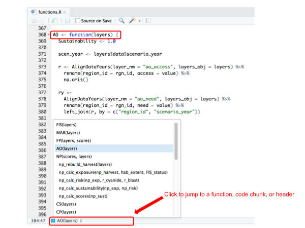
When you modify an individual goal model, you will only work within that function's curly braces `{ }`.

The following things happen in each goal model:
  
  - set scenario year variable and any other constant variables
  - load specific data layers with `ohicore::AlignDataYears()` (recommended over the depreciating `ohicore::SelectLayersData()`) 
  - calculate Status scores 
  - calculate Trend scores 
  - combine Status and Trend scores 
  - format and return the `scores` object

Throughout `functions.R`, you will see syntax from the `tidyverse` package that you installed and loaded. It contains the commonly used data-wrangling functions you'll need in almost every analysis, and enables chaining: `%>%`. To learn more, take a look at [tidyverse.org](http://tidyverse.org/). This [cheatsheet](https://www.rstudio.com/wp-content/uploads/2015/02/data-wrangling-cheatsheet.pdf) is also a helpful guide with quick references to each function. 

> **Tip**: changes must be saved before it is recorded by Git and reflected in the Git window. When new changes are made, the title of your R script will be shown in red color with an *. It will change back to black once the changes are saved. 

Now that we've had this overview looking at this goal model, let's run the code. Remember, we have already loaded the libraries we need, and run the Configure Toolbox code. 

### Load specific data layers with `AlignDataYears()`

`AlignDataYears()` is an `ohicore` function to call the appropriate data layers by its layer name registered in `layers.csv` (e.g. `ao_access`). **Note**: previous versions of the Toolbox use the function `SelectLayersData()`, which still operates correctly, but only for assessments for single years. As we have updated the Toolbox to streamline repeated assessments, `AlignDataYears()` is the preferred function to use.

Run the first few lines of code and the `ao_access` and `ao_need` layers will be loaded, joined into an `ry`, and ready to be manipulated further: 

```{r load_data, eval=FALSE}
  Sustainability <- 1.0

  scen_year <- layers$data$scenario_year

  r <- AlignDataYears(layer_nm = "ao_access", layers_obj = layers) %>%
    rename(region_id = rgn_id, access = value) %>%
    select(-layer_name) %>%
    na.omit()

  ry <-
    AlignDataYears(layer_nm = "ao_need", layers_obj = layers) %>%
    rename(region_id = rgn_id, need = value) %>%
    select(-layer_name) %>%
    left_join(r, by = c("region_id", "scenario_year"))
```

It's always a good idea to check what your data looks like and make sure there are no glaring errors. We can explore what this `ry` object using functions like `head()`, `summary()`, and `str()`. We can write this in the console, or we can add it to the `functions.R` directly (although I would probably comment it out after I'm done testing).

```{r inspect, eval=FALSE}
head(ry)
summary(ry)
str(ry)
```
  
At this point you have probably spent a lot of time preparing these data, but errors can still arise. Things that I would look for: are there NA's? Do I expect them? 

### Goal models

The goal model that was developed for global assessments and described in Halpern et al. 2012 (see current Supplemental Information [here](http://htmlpreview.github.io/?https://github.com/OHI-Science/ohi-global/published/documents/methods/Supplement.html#61_artisanal_opportunities)) states that the status for this goal is represented by unmet demand (Du), which includes measures of opportunity for artisanal fishing, and the sustainability of the methods used. 

$$
D_{U} = (1 - need) * (1 - access)
$$
$$
status = (1 - D_{U}) * sustainability
$$

And this is how it looks in `R`:

```{r ao goal model, eval=FALSE}
 ## model
  ry <- ry %>%
    mutate(Du = (1 - need) * (1 - access)) %>%
    mutate(status = (1 - Du) * Sustainability)
  # head(ry); summary(ry)
```

### Calculate Status 

The status operation in this model is largely filtering out just the recent year of all the years you have calculated in the model above. 

```{r, eval=FALSE}
# status
  ao_status <- ao_model %>%
    dplyr::filter(year==status_year) %>%
    dplyr::select(region_id, status) %>%
    dplyr::mutate(status=status*100)
```

### Calculate Trend 

Next is the Trend scores. They are typically based on linear regression of status scores from the most recent five years (inspect the `trend_years` object below to confirm!). The trend is calculated with the `CalculateTrend()` function from `ohicore`.

```{r, eval=FALSE}
  # trend
  trend_years <- (scen_year - 4):(scen_year)

  r.trend <- CalculateTrend(status_data = ry, 
                            trend_years = trend_years)
```

We can inspect `r.trend`: it returns a dataframe with 3 columns: region_id, score, and dimension.

### Scores variable: combining Status and Trend

Combining the Status and Trend into the scores variable involves selecting only the `region_id` and `score` columns, and adding two more columns identifying score dimension (Status or Trend) and goal name. 

```{r, eval=FALSE}
# return scores
  scores <- rbind(r.status, r.trend) %>%
    mutate(goal = 'AO')
```

The scores variable is something that you'll see at the end of every goal model. Each function ends with returning the `scores` variable, so that `ohicore` can combine all scores together when `CalculateAll()` runs (but we won't run `return(scores)` now. The `scores` variable has a specific format, with four columns. 

```
   region_id    score dimension goal
1          1 94.93492    status   AO
2          2 94.93492    status   AO
3          3 94.93492    status   AO
4          4 94.93492    status   AO
5          5 94.93492    status   AO
6          6 94.93492    status   AO
7          7 94.93492    status   AO
8          8 94.93492    status   AO
9          1  0.01270     trend   AO
10         2  0.01270     trend   AO
11         3  0.01270     trend   AO
12         4  0.01270     trend   AO
13         5  0.01270     trend   AO
14         6  0.01270     trend   AO
15         7  0.01270     trend   AO
16         8  0.01270     trend   AO
```

### Recap of exploring `functions.R`

`functions.R` is a collection of goal models to calculate Status and Trend. Each goal is written inside an `R` function and can have the following steps: 

- set scenario year variable and any other constant variables
- load specific data layers with `ohicore::AlignDataYears()` (recommended over the depreciating `ohicore::SelectLayersData()`) 
- calculate Status scores 
- calculate Trend scores 
- combine Status and Trend scores 
- format and return the `scores` object


## Calculate with tailored models

Now let's run through the basic workflow a third time, this time modifying a goal model but keeping all data layers the same. We will do this without making any changes to the data layers at the moment. Tailoring a goal model involves editing the operations within that goal's model in `functions.R`. 

![](https://docs.google.com/drawings/d/1VRckHItA151selmkBVtROk6OnLnI_ODIu2gIjSnFgmo/pub?h=450)

### Restart R, Libraries, Configure Toolbox 
 
First let's restart `R` and rerun the Load Libraries and Configure Toolbox sections in `calculate_scores.Rmd`. Now, we are all set to dive into the models in `functions.R`.

### Tailor AO goal model

Now, let's go to `functions.R`, to the AO model. As an example, we will do something pretty simple to tailor the goal model. Let's say we just wanted to divide the variable `Du` by 2 in the equation. 

```{r tailor AO goal model, eval=FALSE}
  # model
  ry <- ry %>%
    mutate(Du = (1 - need) * (1 - access)) %>%
    mutate(status = (1 - Du/2) * Sustainability)
```

We can run the rest of the AO function line-by-line and inspect the scores variable at the end to see if everything looks OK. 

### Calculate scores, check, plot, and sync

Now let's run the Calculate Scores chunk and save `scores.csv`. 

We can use Git's differencing feature to see how our scores have changed. This is a great way to double-check and error-check that things are working the way you expected. 

We can also recreate the flower plots with our updated goal model. Then let's commit and sync so we can see the differences on GitHub.com. 

My commit message here will be "toolbox-training: tailor AO goal model with original data layer". 

### Recap of third `calculate_scores.Rmd` run

In this third time through the basic workflow, we updated the goal model without changing any of the data layers that it depends upon. Next up, we will add a new data layer for it to work with.


### Troubleshooting

If you've tailored a goal model function, you need to make sure that its output is still a data frame, and one that is not grouped. Otherwise, when you run `calculate_scores.Rmd`, you may get a cryptic error. Examples of some of the ones we've seen are: 

```{r, eval=FALSE}
# Error in left_join_impl(x, y, by$x, by$y, suffix$x, suffix$y, check_na_matches(na_matches)) : 
#  Can't join on 'region_id' x 'region_id' because of incompatible types (integer / list)
```

We are constantly improving `ohicore` with more human-readable error messages, but it is still best practice to ensure your goal model output is returning a dataframe. 

You can do this in a few ways. The way we commonly do this is by adding `ungroup()` or `as.data.frame()` as the final step before returning the scores variable at the end of a goal model function. 

## Calculate with tailored data and models
 
The fourth and final example we will do in this chapter is to tailor a goal model by adding a new variable. This will mean that we will prepare, save, and register a *new* data layer and update the goal model in `functions.R`. It will be a combination of what we've done previously in this chapter. 

Let's restart `R` before proceeding.

![](https://docs.google.com/drawings/d/e/2PACX-1vQ7Ws3tiltTDeBhaoQy2naem8slDq297boGkgTaSC2n8SoJOKyDtXl5Hy-0obnRuRfY8-xB24PskRq3/pub?w=960&h=720)

Let's say, as an example, that we want to tailor the AO goal model by adding a new variable for *poverty* into the equation.

$$
D_{U} = (1 - (need + poverty) / 2) * (1 - access)
$$
$$
status = (1 - D_{U}) * sustainability
$$


### Prepare and save our new data layer

We will create the new data layer for poverty by running a script in the prep folder. 

Open `toolbox-demo/prep/AO/poverty_prep.R` and source the file after reading it through. The result will be a new data layer saved to the "layers" folder, and you should see that there is a new file saved in your Git window. 

### Register in `layers.csv` 

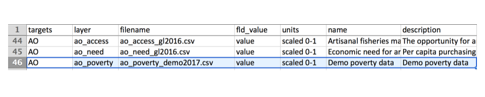
Now that we have prepared and saved our data layer, we'll register it in `layers.csv`. This time, since we have added an additional data layer that has not been previously registered, we need to add a new row. 

Open `region2017/layers.csv` in a spreadsheet software (i.e. Microsoft Excel or Open Office). Add a new row for "ao_poverty", and fill in the following information. We've added the row near the other AO data layers.

![](https://docs.google.com/drawings/d/1n9qMQuyOxfkZzTGgj2vGaGY7YwS_A3PMtDAjaKfc3Co/pub?w=960&h=192)


### Register in `scenario_data_years.csv` 




### Configure Toolbox

To use this layer as we develop our goal model, we need to rerun the Configure Toolbox section. Before that, let's restart R, and reload the libraries. It's good to restart R often so that you don't introduce errors later (that could be because your work is dependent on something that shouldn't be there, like in our layer preparation). 

### Update the AO goal model

We will need to do two things to update the goal model in `functions.R`.

First, we'll have to load our data layer with `AlignDataYears()`. You can copy-paste the following into your `functions.R` to make sure everything is working properly:

```{r SelectLayersData pov, eval=FALSE}
  Sustainability <- 1.0

  scen_year <- layers$data$scenario_year

  r <- AlignDataYears(layer_nm = "ao_access", layers_obj = layers) %>%
    rename(region_id = rgn_id, access = value) %>%
    select(-layer_name) %>%
    na.omit()
  
  rp <- AlignDataYears(layer_nm = "ao_poverty", layers_obj = layers) %>%
    rename(region_id = rgn_id, poverty = value) %>%
    select(-layer_name) %>%
    left_join(r, by = c("region_id", "scenario_year")) 

  ry <-
    AlignDataYears(layer_nm = "ao_need", layers_obj = layers) %>%
    rename(region_id = rgn_id, need = value) %>%
    select(-layer_name) %>%
    left_join(rp, by = c("region_id", "scenario_year")) 
```

Let's run this and inspect the variables. 

*Note*: if you forgot to add `ao_poverty` as a new layer to `scenario_data_years.csv` in the section above, you wouldn't get an error, but when your `rp` variable wouldn't read any any data, it would be a dataframe with 0 rows! That is why it's important to inspect all these variables so you can trace back where the problem is as early as possible. 

Alright. Next, we'll tailor the goal model itself. Here is how the goal model looks as an equation and in `R`: you can copy-paste this model into `functions.R`, replacing the existing model.

$$
D_{U} = (1 - (need + poverty) / 2) * (1 - access)
$$

$$
status = (1 - D_{U}) * sustainability
$$

```{r tailored ao goal model, eval=FALSE}
## tailored goal model with poverty
ry <- ry %>%
    mutate(Du = (1 - (need + poverty) / 2 ) * (1 - access)) %>%
    mutate(status = (1 - Du) * Sustainability)
```

### Calculate scores, check, and sync

Everything is looking good in `functions.R` and in the Git tab that we're looking at as we go along. 

Now let's restart `R` and recalculate scores  in `calculate_scores.Rmd`. We'll see that `scores.csv` will also update, and we can check that only AO dimensions (except pressures and resilience since we haven't changed them) and Index scores are affected. 

Let's commit and sync. My commit message will be "toolbox-training: tailor AO goal model with a new data layer".

### Recap of fourth `calculate_scores.Rmd` run

In this run we combined what we have practiced in the previous two runs, and we successfully: 

- created a new data layer, which includes preparing layer in the prep file, saving it in `layers`, and registering it in `layers.csv` and `scenario_data_years.csv`
- added this new model variable (ie. new layer) in AO model in `functions.R`
- reran `calculate_scores.Rmd` and saw the changes reflected in Git

## Chapter Recap

We have completed Chapter \@ref(calcs-basic) and successfully run through the basic workflow to calculate OHI scores with several variations using our **toolbox-demo** repository. 

Each variation involves the same basic workflow of bookkeeping and running `calculate_scores.Rmd`, and will enable you to begin tailoring the Toolbox for your assessment.

1. 'out of the box' data and models extracted from the Global 2016 assessment
1. tailored data and 'out of the box' models
1. tailored data and models
1. tailored (new) data and models

![](https://docs.google.com/drawings/d/e/2PACX-1vQ7Ws3tiltTDeBhaoQy2naem8slDq297boGkgTaSC2n8SoJOKyDtXl5Hy-0obnRuRfY8-xB24PskRq3/pub?w=960&h=720)

Also, a few **best practices** we have used throughout this training that are good to remember: 

- Compulsively restart R
- Always check Git window after each change for expected changes
- Commit, then Pull before Push
- Rerun the Configure Toolbox code chunk after any data layer or model changes
- Save `functions.R` before the changes are reflected in Git window 
- Close Excel before returning to `R` (this is less important on a Mac but will cause errors on a PC)



<!---next steps after March 1 training: 

## Update pressures and resilience matrices

- PlotFlower, PlotMap
- updating pressures/resilience matrices
- goals.csv and preindex function...
- see https://cdn.rawgit.com/OHI-Science/ohi-science.github.io/dev/assets/downloads/pres/tutorial_tbx_modifications.html
--->