Author: Behrouz Safari
License: MIT
A python package for retrieving and analysing data from SDSS (Sloan Digital Sky Survey)
Important:
CSV
Install the latest version of sdss from PyPI:
pip install sdss
Requirements are numpy, requests, Pillow, matplotlib, pandas and astropy. Versions before 1.0.0 are not dependent on astropy.
Let's create a Region:
from sdss import Region

ra = 179.689293428354
dec = -0.454379056007667

reg = Region(ra, dec, fov=0.033)
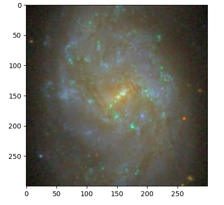
To see the image:
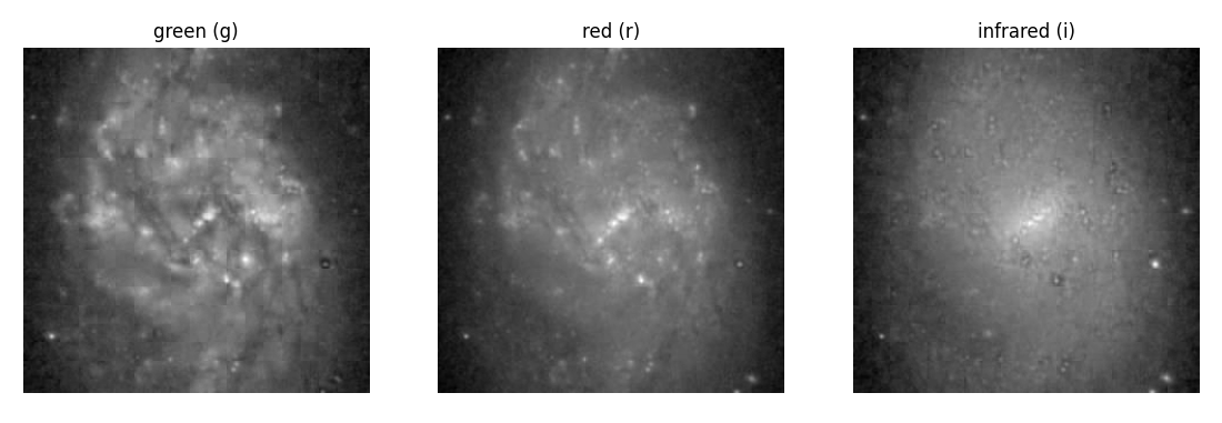
reg.show()To see the image in three gri filter bands (green, red, infrared) separately:
reg.show3b()To find nearest objects:
df_obj = reg.nearest_objects()To find nearest objects with spectrum:
df_sp = reg.nearest_spects()Let's download a frame, in fits and jpg, retrieve all of its objects.:
from sdss.photometry import frame_filename, obj_frame_url, \
     download_file, unzip, get_df, df_radec2pixel

objid = 1237646587710014999

zip_file = 'data/' + frame_filename(objid) + '.fits.bz2'
fits_file = zip_file[:-4]
jpg_file = fits_file.replace('-r-', '-irg-').replace('fits', 'jpg')

zip_url = obj_frame_url(objid, 'r')
download_file(zip_url, 'data/')
unzip(zip_file)

jpg_url = obj_frame_url(objid, 'irg', jpg=True)
download_file(jpg_url, 'data/')

df = get_df(objid)
df = df_radec2pixel(df=df, fits_file=fits_file)

df.to_csv('data/COMP.csv', index=False)
Now we can plot our target image:
import pandas as pd
import matplotlib.pyplot as plt
from sdss.photometry import frame_filename, obj_from_jpg

objid = 1237646587710014999

jpg_file = 'data/' + frame_filename(objid).replace('-r-', '-irg-') + '.jpg'

df = pd.read_csv('data/COMP.csv')

img = obj_from_jpg(jpg_file=jpg_file, df=df, objid=objid)

fig, ax = plt.subplots()
ax.imshow(img)
plt.show()
Let's find the best apparture:
from sdss.photometry import flux

data = img[:,:,0]
half = data.shape[0]//2
center = (half, half)

ls_r_star = [2, 3, 4, 5, 6, 7, 8, 9, 10, 11, 12]
ls_background = []
ls_real_flux = []
for r_star in ls_r_star:
    background, real_flux = flux(data, center, r_star)
    ls_background.append(background)
    ls_real_flux.append(real_flux)

fig, ax = plt.subplots()
ax.scatter(ls_r_star, ls_real_flux, c='b')
ax.set_xlabel('R star')
ax.set_ylabel('Sky subtracted flux')
plt.grid()
plt.show()
See more examples at astrodatascience.net

