Measuring a solution

Once a solution for one of scheduling models presented here has been devised, different measures of the merits of the solution can be obtained. These are of two types:

• Measures at job-machine level
• Measures at job level

Job-machine level measures

There are two basic job-machine level indicators of a solution. The first one is ct, which provides a list of the completion time of each job on each machine. Therefore ct[i][j] indicates the completion time on machine i of the job provided in the solution in order j. For most of the basic scheduling models included in the library, the solution is given in the form of a sequence of jobs, but it is not always the case (for instance, for the JobShop and OpenShop models, that use different solution encodings). Therefore, along with the completion times of the jobs on the machines, the order in which the jobs are presented in the list of completion times should be given. This is particularly important in the case of partial solutions (i.e. solutions that only contain some of the jobs to be scheduled). Let us consider the following example for the SingleMachine environment:

from scheptk.scheptk import SingleMachine

instance = SingleMachine('test_single.txt')
sequence = [2,1]
completion_times, job_order = instance.ct(sequence)

print(completion_times)
print(job_order)

Note that the solution provided in sequence is a partial sequence, as it contains jobs 1 and 2, but no job 0 (and possible other jobs). If the file test_single.txt contains the following tags: [JOBS=4] and [PT=2,10,1,1], then the result of the above code is the following:

[[1, 11]]
[2, 1]

The first line (the printing of completion_times) contains a list with one row with two columns. Therefore ct[0][0] contains the completion time on the first (and only) machine of the first job in the solution (job 2), whose processing time is 1. The ct[0][1] contains the completion time on the first machine of the second job in the solution (job 1), whose processing time is 10 (which results in a completion time of 1 + 10 = 11). The second line (the printing of job_order) contains an order that indicates what job corresponds to each row in ct. In the example, it indicates that the first column in the list in ct corresponds to the completion times of job 2, whereas the second column contain the completion times of job 1.

While for some models (i.e. SingleMachine, ParallelMachines,UnrelatedMachines and FlowShop), job_order is the same as the solution provided, this is not true for JobShop and OpenShop models, which have extended solution encoding. Note the following code:

from scheptk.scheptk import OpenShop

instance = OpenShop('test_openshop.txt')
sol = [7,5,4,0,1,6,3,2,8]
print(sol)
ct, order = instance.ct(sol)

print(ct)
print(order)
instance.print_schedule(sol)

When the data in test_openshop.txt are given by the following tags:

[JOBS=3]
[MACHINES=3]
[PT=10,5,18;15,20,6;10,16,8]

then the output is

[7, 5, 4, 0, 1, 6, 3, 2, 8]
[[41, 59, 10], [36, 6, 51], [16, 67, 26]]
[1, 2, 0]

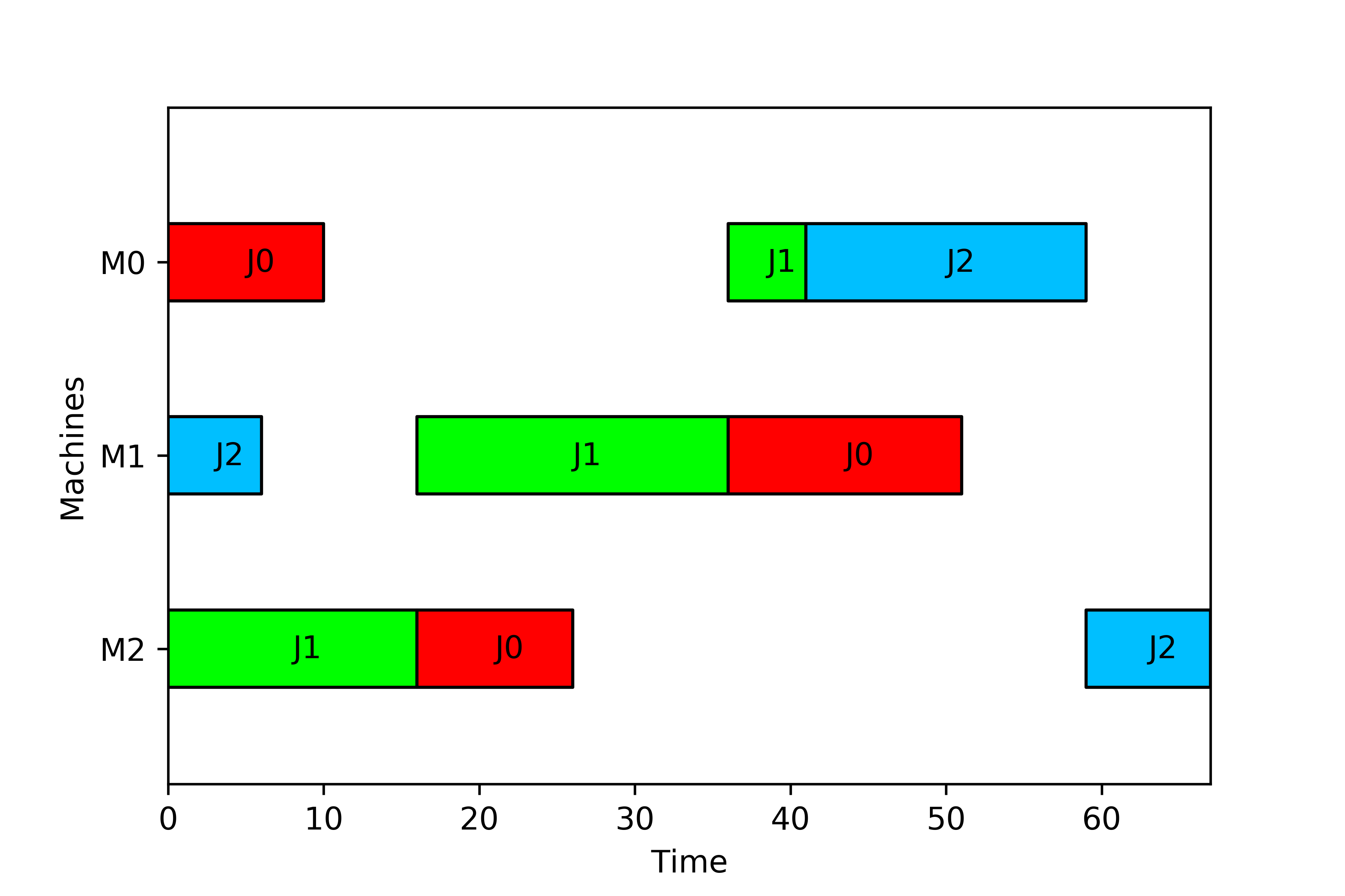
and the figure

In this case ct[0][0] contains the completion time on machine 0 of the first job in the order given by order (i.e. job 1), and e.g. ct[1][2] contains the completion time on machine 1 of the third job in the order given by order (i.e. job 0). As we can see, in this case the information given in order is useful, as the solution sol does contain operations and not jobs, and therefore the job order is not clear in the solution.

Whenever one job is not processed in some specific machine (as, for instance, it happens in the ParallelMachines and UnrelatedMachines) models, the corresponding processing times in ct are zero.

Using ct and particularly returning the job order may seen a bit complex but it allows us to handle partial solutions (as we have seen in the SingleMachine example) in a compact manner, as otherwise the completion times of the jobs in ct would be hard to express, since job 0 is not in the partial solution and therefore ct[0][0] cannot indicate the completion time on machine 0 of job 0.

An alternative to ct is the method ctn, which provides the completion time of all the jobs in the machines. Here ct[i][j] indicates the completion time on machine i of the job j. If job j has not been scheduled (because i.e. the solution is a partial solution), then a nan (not available number) is returned in its place. Therefore, the following code:

from scheptk.scheptk import SingleMachine

instance = SingleMachine('test_single.txt')
sequence = [2,1]
completion_times, job_order = instance.ct(sequence)

print(completion_times)
print(instance.ctn(sequence))

when the test_single.txt instance contains the same data as above produces the following output:

[[1, 11]]
[[nan, 11, 1, nan]]

Note the difference between the completion times provided by ct and those provided by ctn: ctn[0][0] indicates the completion time on machine 0 of job 0. Since job 0 is not part of the solution provided, its completion time is nan. ct[0][1] contains the completion time of job 1 on machine 0. This job is the second job in the partial solution provided, hence its completion time is higher than that of job 2 (which is the first job provided in the partial solutions).

A final, additional example is provided next for the UnrelatedlMachines model. The following code

from scheptk.scheptk import UnrelatedMachines

instance = UnrelatedMachines('test_unrelated.txt')
sequence = [2,5,0,4]
ct, order = instance.ct(sequence)
print(ct)
print(instance.ctn(sequence))
instance.print_schedule(sequence, 'unrelated_partial_sample.png')

with the data given in the tags [JOBS=6], [MACHINES=2], [PT=5,13,5,2,8,6;9,12,10,4,3,10] yields the following results

[[5, 0, 10, 0], [0, 10, 0, 13]]
[[10, nan, 5, nan, 0, 0], [0, nan, 0, nan, 13, 10]]

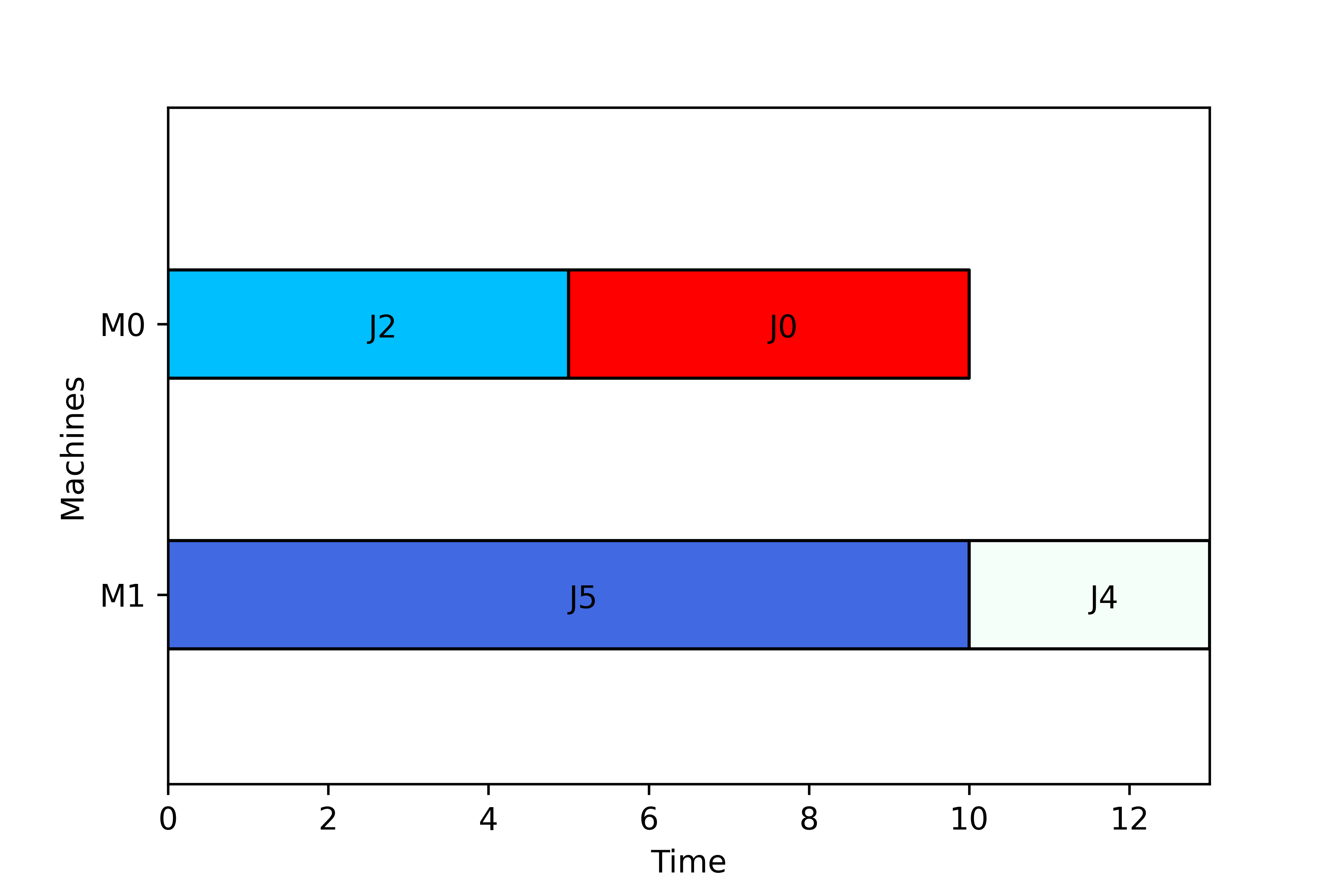
and the following figure

A final remark on ct and ctn

As we have seen, information regarding the completion times is provided by the functions in scheptk using two alternatives, ct and ctn. Both approaches have pros and cons, and whereas it is clear that ct provides a more compact way to handle partial solutions and the information is clearer in scheduling models whose solution encoding consists of a sequence, the interpretation is more confusing than ctn for JobShop, OpenShop models, or models with sophisticated solution encodings. scheptk provides both, so it is up to the user to pick the one that fits better for him/her.

Job-level measures

Job-level measures usually aggregate (or combine with additional data) job-machine level measures. Job-level measures can be computed using a number of methods described below, and indeed these methods are internally called by the models to obtain scheduling criteria.

The most classical job-level measure are the completion times of the jobs in a solution. These can be obtained with the method Cj(solution) that returns a list of the completion times of each job in the solution in the order of the jobs provided in the solution. More specifically, the following code

from scheptk.scheptk import SingleMachine
instance = SingleMachine('test_single.txt')
completion_times = instance.Cj( [2,0] )
print(completion_times)

for the instance with tags [JOBS=4] and [PT=2,10,1,1] yields the following output:

[1, 3]

which corresponds to first processing job 2 (with processing time 1) and then job 0 (with processing time 2). Therefore completion_time[0] contains the completion time of the first processed job (job 2) while completion_time[1] contains the completion time of the second processed job (job 0).

In the same manner than ct and ctn in the section above, an alternative to obtain the completion times of the jobs is to use the method Cjn(solution) --note the difference of the n--, which provides the completion time of all jobs (even if they are not part of the solution) in the natural job order. More specifically, just changing the third line in the code above by completion_times = instance.Cjn( [2,0] ), the following output is produced:

[3, nan, 1, nan]

which indicates that job 0 has a completion time of 3, that job 1 is not part of the solution and hence its completion times are not available (nan), that job 2 has a completion time of 1, and that job 3 is not part of the solution.

Similarly to the completion times, the following additional methods are available to compute job-level measures:

• Ej(solution) - returns a list with the earliness of each job in solution. The order of the values is that of the jobs in solution (as in Cj).
• Ejn(solution) - returns a list with the earliness of all jobs according to solution. The order of the values is the natural order (as in Cjn).
• Fj(solution) - returns a list with the flowtime of each job in solution. The order of the values is that of the jobs in solution (as in Cj).
• Fjn(solution) - returns a list with the flowtime of all jobs according to solution. The order of the values is the natural order (as in Cjn).
• Lj(solution) - returns a list with the lateness of each job in solution. The order of the values is that of the jobs in solution (as in Cj).
• Ljn(solution) - returns a list with the lateness of all jobs according to solution. The order of the values is the natural order (as in Cjn).
• Sj(solution) - returns a list with the starting time in the system of each job in solution. The order of the values is that of the jobs in solution (as in Cj).
• Sjn(solution) - returns a list with the starting time in the system of all jobs according to solution. The order of the values is the natural order (as in Cjn).
• Tj(solution) - returns a list of with tardiness of each job in solution. The order of the values is that of the jobs in solution (as in Cj).
• Tjn(solution) - returns a list of with tardiness of all jobs according to solution. The order of the values is the natural order (as in Cjn).
• Uj(solution) - returns a list indicating if a job in solution is tardy (1), or not (0). The order of the values is that of the jobs in solution (as in Cj).
• Ujn(solution) - returns a list indicating if each job is tardy (1), or not (0), according to solution. The order of the values is that of the jobs in solution (as in Cj).