README.md

This library provides objects that model probability distributions and the related operations that are common in generative Bayesian modeling and Bayesian inference, including Gibbs sampling and variational mean field algorithms. The file abstractions.py describes the queries a distribution must support to be used in each algorithm, as well as an API for models, which compose the distribution objects.

Example

The file models.py shows how to construct mixture models building on the distribution objects in this library. For example, to generate data from a Gaussian mixture model, we might set some hyperparameters, construct a Mixture object, and then ask it to randomly generate some data from the prior:

import numpy as np
from pybasicbayes import models, distributions

# hyperparameters
alpha_0=5.0
obs_hypparams = dict(mu_0=np.zeros(2),sigma_0=np.eye(2),kappa_0=0.05,nu_0=5)

# create the model
priormodel = models.Mixture(alpha_0=alpha_0,
        components=[distributions.Gaussian(**obs_hypparams) for itr in range(30)])

# generate some data
data = priormodel.rvs(400)

# delete the model
del priormodel

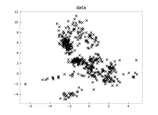
If we throw away the prior model at the end, we're left just with the data, which look like this:

from matplotlib import pyplot as plt
plt.figure()
plt.plot(data[:,0],data[:,1],'kx')
plt.title('data')

Imagine we loaded these data from some measurements file and we wanted to fit a mixture model to it. We can create a new Mixture and run inference to get a representation of the posterior distribution over mixture models conditioned on observing these data:

posteriormodel = models.Mixture(alpha_0=alpha_0,
        components=[distributions.Gaussian(**obs_hypparams) for itr in range(30)])

posteriormodel.add_data(data)

Since pybasicbayes implements both Gibbs sampling and variational mean field inference algorithms, we can use both together in a hybrid algorithm.

import copy
from pybasicbayes.util.text import progprint_xrange

allscores = [] # variational lower bounds on the marginal data log likelihood
allmodels = []
for superitr in range(5):
    # Gibbs sampling to wander around the posterior
    print 'Gibbs Sampling'
    for itr in progprint_xrange(100):
        posteriormodel.resample_model()

    # mean field to lock onto a mode
    print 'Mean Field'
    scores = [posteriormodel.meanfield_coordinate_descent_step()
                for itr in progprint_xrange(100)]

    allscores.append(scores)
    allmodels.append(copy.deepcopy(posteriormodel))

import operator
models_and_scores = sorted([(m,s[-1]) for m,s
    in zip(allmodels,allscores)],key=operator.itemgetter(1),reverse=True)

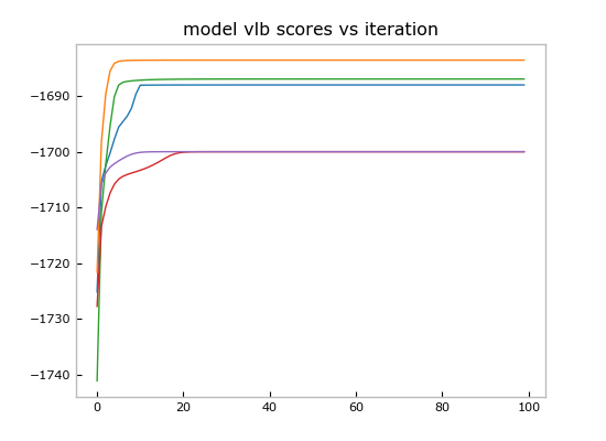
Now we can plot the score trajectories:

plt.figure()
for scores in allscores:
    plt.plot(scores)
plt.title('model vlb scores vs iteration')

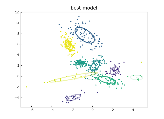
And show the point estimate of the best model by calling the convenient Mixture.plot():

models_and_scores[0][0].plot()
plt.title('best model')

Since these are Bayesian methods, we have much more than just a point estimate for plotting: we have fit entire distributions, so we can query any confidence or marginal that we need.

See the file demo.py for the code for this demo.

Authors

Matt Johnson, Alex Wiltschko, Yarden Katz, Nick Foti, and Scott Linderman.