

- Demo
- Setup
- Start application
- Preparing your own data
- Configuration
- The gGnome.js interface
- Genome graph JSON format description
- Adding description of your samples
- FAQ
If you wish to use gGnome.js to explore data from Hadi et al. 2020, you can use this link. You can also find some demo data to play demonstrating the different features of the interface at the following location.
gGnome.js runs in a web browser. We recommend using Google Chrome since that's what we used when testing the application. It should work on other browsers too, but we make no promises.
For execution, you will only need Node.js installed on your environment. Notice that gGnome.js has only been tested on unix systems (MacOS, Linux).
Node is really easy to install and now includes NPM. You should be able to run the following command after the installation procedure below:
$ node --version
v0.10.24

$ npm --version
1.3.21
Please install Homebrew if it's not already done with the following command:
$ ruby -e "$(curl -fsSL https://raw.github.com/Homebrew/homebrew/go/install)"
If everything when fine, you should run
brew install node
sudo apt-get install python-software-properties
sudo add-apt-repository ppa:chris-lea/node.js
sudo apt-get update
sudo apt-get install nodejs
Just go on official Node.js website & grab the installer.
Also, be sure to have git available in your PATH, npm might need it. Notice that gGnome.js has only been tested on unix systems (MacOS, Linux). It should work on Windows too, but has not been fully tested on Windows. If you run into trouble then please let us know.
$ git clone git@github.com:mskilab/gGnome.js.git
$ cd gGnome.js/
$ npm install
In order to use the application, you must have the reference JSON files: genes.json and metadata.json under the public subdirectory inside the gGnome.js directory. If you are using hg19, then the genes.json file will be downloaded automatically for you upon the first launch of the application and you can skip this section. If from some reason the hg19 genes.json file did not download automatically then you can run this command:
wget -P public/ https://mskilab.s3.amazonaws.com/pgv/genes.json
Notice that the default reference file for hg19 does not include 'chr' as a prefix in sequence names. If your data includes the 'chr' prefix ('chr1', 'chr2', ...), then you need to download the hg19_chr reference and replace the existing gene.json with this file. To do so, run the following command from inside your gGnome.js directory:
wget -O public/genes.json https://mskilab.s3.amazonaws.com/pgv/hg19_chr.genes.json
mv public/metadata_chr.json public/metadata.json
If you are using hg38 (no chr prefix), then run the following command to download the hg38 reference file:
wget -O public/genes.json https://mskilab.s3.amazonaws.com/pgv/hg38.genes.json
cp public/hg38/metadata.json public/
And if you are using hg38 and the sequence names in your data include the 'chr' prefix, then run:
wget -O public/genes.json https://mskilab.s3.amazonaws.com/pgv/hg38_chr.genes.json
cp public/hg38/metadata_chr.json public/
In the project folder, you may initiate the application via the terminal:
$ ./start.sh
In case it doesn't start automatically, open your preferred browser and navigate to the url
http://localhost:8080/index.html
The validation of the data.json files is available at the respective Validator page
http://localhost:8080/validator.html
The gGnome package includes tools for producing all required data for visualization with gGnome.js. More details are available in this section of the gGnome tutorial.
The application is reading
- the intervals, the walks, and their connections from the json file in gGnome.js/json/data.json
- the genes from the json file in gGnome.js/json/genes.json
- the chromosome metadata from the json file in gGnome.js/json/metadata.json
In order to test your own data, simply replace the file gGnome.js/json/data.json with your own, on condition you maintain the same structure
Once you launch the interface (following the instructions above), you should see something like this:
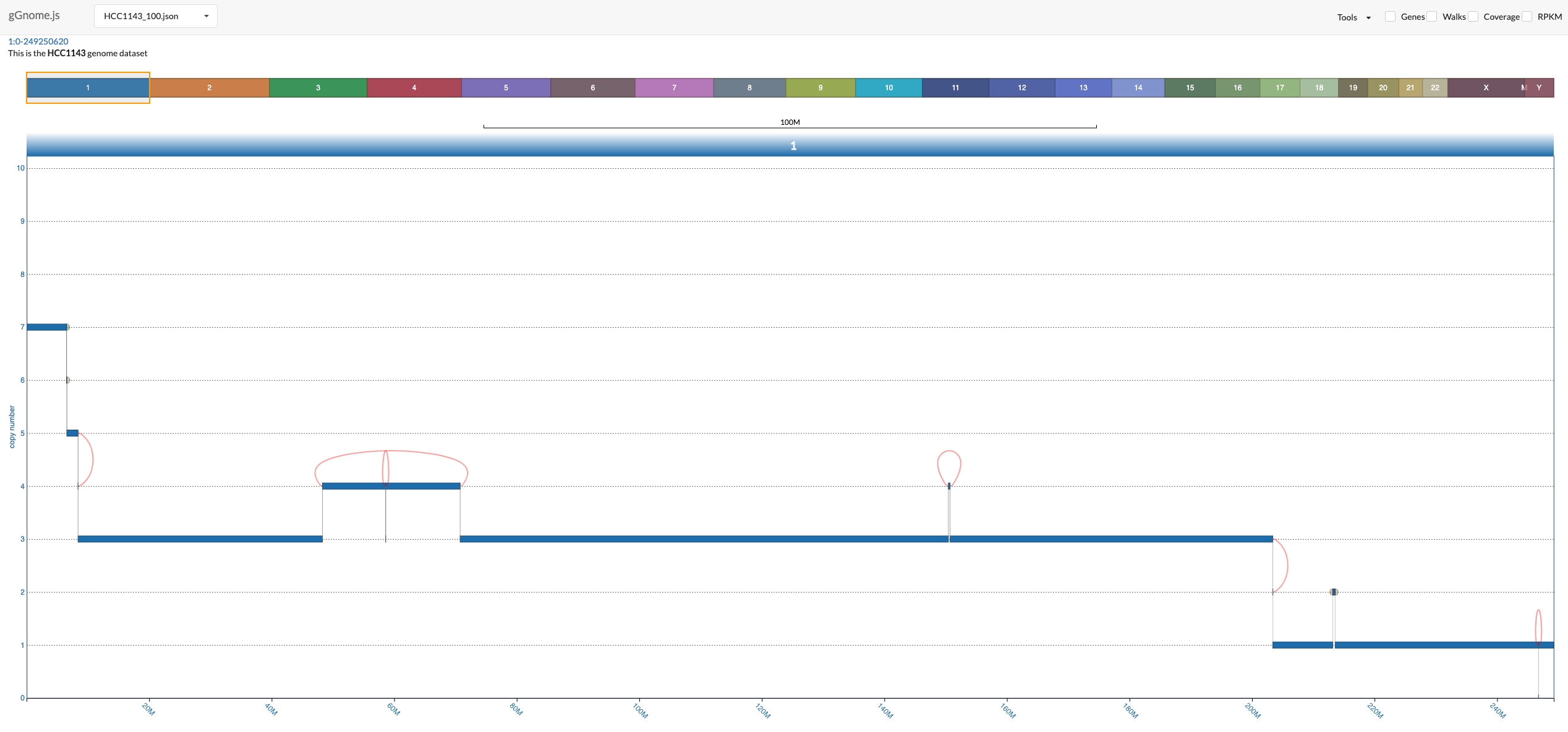
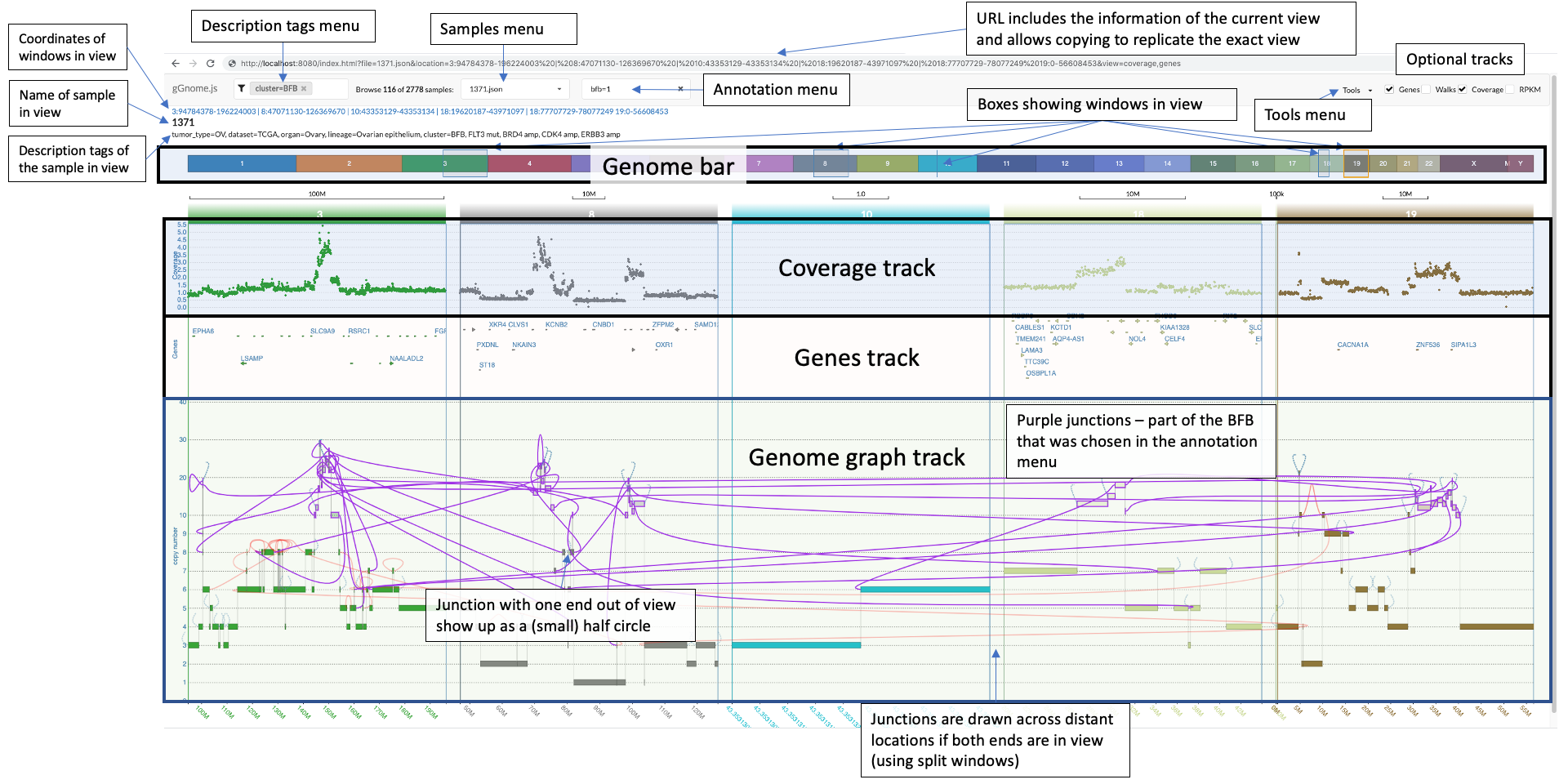
There is a lot to unfold so the following image includes overview of the components in the interface:
In the bottom, you see the genome graph, where each node of the graph (representing a segment of the genome) is plotted with the y-axis position according to the values in the JSON file. The red edges between nodes are "ALT" junctions, and the black edges are "REF" junctions.
When you hover above nodes and edges you can see some information:


The genome bar shows you which segments of the genome are currently in view. Notice that you can have multiple split windows showing separate locations across the genome. You can open a new split window by clicking and dragging the mouse pointer on a location in the genome bar.
There are multiple ways to change the zoom. You can modify the width of each individual window in the genome bar by clicking on one of it's sides and dragging it, or you can use the mouse scroll when positioning the mouse pointer above the genome graph track. Similarly, you can also click and drag each window (both in the genome bar and in the genome graph track).
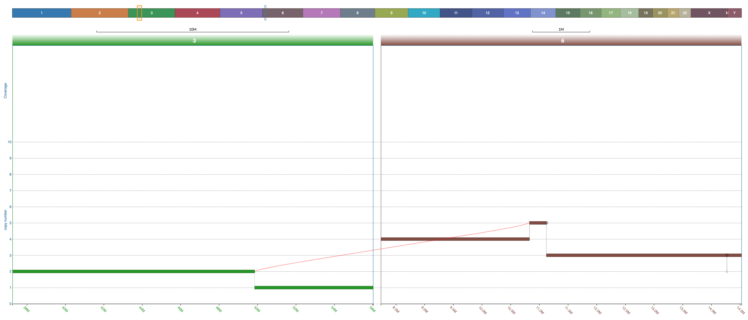
Notice that junctions are drawn only if both ends of the junction are currently in view, but the ends of the junction can be in different windows (this allows you to focus on specific junction/s even when the nodes it connects are distant:
If only one end of a junction is in view then a half circle would appear where the junction should be. If you double click on that half circle then a split window containing the other end of the junction would appear and thus the junction would be shown. This is extremely useful.
The arrows in the screenshot below highlight the two half circles representing junctions each with one end out of vision:

The top bar includes for options for you to choose from:

You can browse the various samples available in your project using the dropdown menu on the top left:

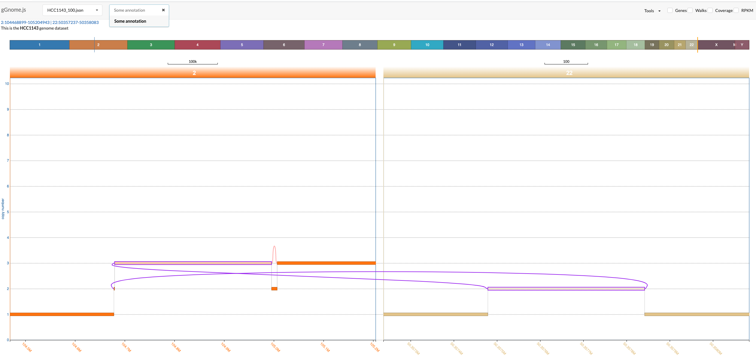
If your sample includes annotations (see JSON format description below), then an additional dropdown menu from which you can choose an annotation to focus on. Once you click on a specific annotation then gGnome.js would automatically adjust the zoom to focus on all intervals and connections that were annotated with the specific annotation. These intervals and connections would also be highlighted in purple:
The most common use for annotations is to annotate nodes and edges with SV annotations as described in the gGnome tutorial
On the top right of the interface there are optional tracks that could be shown or hidden:
- Genes - this track shows the location of genes as arrows (pointing in the direction of transcription). When clicking on a gene name you would be directed to the gene card entry for the gene. When hovering over the gene body (the arrows) you can see some information regarding each gene. When clicking on an arrow, a window would pop up showing the location of UTRs and CDSs. Genes are defined inside the gGnome.js directory in
public/genes.json. Instructions on how to make this file from any GTF are coming soon (if this is 2022 and there are no instructions then please contact us). - Walks - if any walks are defined in the JSON file, then this track would show them.
- Coverage - coverage file corresponding to the genome graph. The coverage files are found in the
scatterPlotdirectory. Each coverage file must have a.csvsuffix and correspond in name to the JSON file. For example the genome graphjson/HCC1143_100.jsoncorresponds to coverage filescatterPlot/HCC1143_100.csv. - RPKM - this track is intended for showing RPKM data, but could actually be used to show any arbitrary data in bar plot format. The RPKM files are stored in the
barPlotdirectory. As with the coverage file, the name must correspond to the name of the genome graph JSON file. For example:barPlot/HCC1143_100.csv
At the top right (next to the optional tracks), you can find the "Tools" menu. When you click on it, you have for options:
- Locate - this is a very useful feature! When you click on this a window will open allowing you to search any gene or genomic location and open a new split window focused on that gene or genomic region.
- Validate - you can use this to upload a JSON file and validate that it is formatted correctly.
- Upload - you can use this to upload a CSV of coverage data. But the preferred way to incorporate coverage data is the way described above.
- Export - if you click on this then a copy of the genome graph JSON file will be downloaded. This is useful when browsing data that is hosted on a remote server (e.g. mskilab.com/gGraph)
The genome graph JSON format generally includes the following main fields:
- "settings": these are some general configurations that you can control, such as the title for the y axis and the description that appears on the left top of the screen.
- "intervals": the list of interval (AKA nodes) that define your genome graph
- "connections": the list of connections (AKA edges) in your genome graph
- "walks": the list of walks. Notice that each individual walk is similar in definition to a complete genome graph. So each walk includes a list of connections (titled "cids"), and a list of intervals (titled "iids")
The intervals and connections in the genome graph JSON have a special field called "annotation". The unique list of annotation strings will appear in a dropdown menu at the top left of the interface and when you choose a certain annotation then the interface would automatically adjust the zoom to focus on all nodes and edges that were annotated using the annotation that was chosen. For details on how to use the gGnome package to get annotations of complex structural variation please refer to the gGnome tutorial
You can add some tags to describe various charachteristics of your samples. If added then these are searchable using the description tags menu at the top left of the interface. This is useful for projects in which you have a lot of samples and you wish to be able to take a look at a subset of samples with a certain charachteristic (e.g. BRCA1 mutation).
The tags are provided using a file named datafiles.csv. This file should be placed in the gGnome.js directory and an example file is provided here. Each line corresponds to a sample where the first column should match one of the JSON files in the json subdirectory of the gGnome.js directory and the second column includes your tags deparated by a semicolon and single space (; ).
To close a window click on that window in the genome graph track and then hit the backspace key.