Python Data Analysis Library
A fully-featured code library for manipulating data arranged in tables (i.e. matricies or data frames). It's arguably the most popular Python library used for data engineering. For those of you who have used the popular statistical language, R, Pandas brings many of that languages capabilities to python.
So far we've discussed how you build your own multidimensional objects like lists of lists and dictionaries of dictionaries from raw data. However, bioinformatics modules (and many others) will often return results in the form of Pandas data frame or a matrix. Further manipulation of these results (e.g. filtering, statistical analysis, data reorganization) will require some knowledge of Pandas operations.
-
Open a local file using Pandas, usually a comma-separated values (CSV) file, but could also be a tab-delimited text file (TSV), Excel, json, etc
-
Read a remote file on a website through a URL or read data from a remote database.
A matrix is an data structure where numbers are arranged into rows and columns. They will typically contain floats or integers, but not both. Matrices are used when you need to perform mathematical operations between datasets that contain multiple dimensions (i.e. measurements for two or more variables that change at the same time).
A data frame is a table-like data structure and can contain different data types (strings, floats, integers, etc.) in different columns. This is the type of data structure you're used seeing in Excel. Each column should only contain one data type.
Operations in Pandas, like R, work most efficiently when vectorized
You can think of a vector (also referred to as an array) as a type of list that contains a single data type and optimized for parallel computing. For matricies and data frames in Pandas (also NumPy), vectors are rows and columns.
Rather that looping through individual values (scalars), we apply operations to vectors (rows/columns). That is, the vector is treated as a single object. This topic can get a bit complicated, but it is worth doing your homework if you frequently work with these data types. Here's a few articles to get you started:
- A beginners guide to optimizing pandas code for speed.
- Why is vectorization faster in general than loops?
- Python Lists vs. Numpy Arrays, what's the difference?


Vectorization with Pandas series is ~390x faster than crude looping
Each function (method) in Pandas has many options and might not work the way you expect. It's definitely worth reading the documentation. Functions and options are sometimes updated, so even if you are already familiar with a function, it's a good idea to have a quick look.
Documentation is here https://pandas.pydata.org/docs/
Read getting started first https://pandas.pydata.org/docs/getting_started/index.html#getting-started
(what's possible: data types, summary stats, plots, table layouts, merging)
Pandas user guide (how it works, details on how Pandas thinks about data types) https://pandas.pydata.org/docs/user_guide/index.html#user-guide
Specific information about all the methods and classes https://pandas.pydata.org/docs/reference/index.html#api
But you'll probably want to start with a google search like pd load dataframeor pandas read excel skip rows
import pandas as pd

seq_info_input=pd.read_csv('sequencing_input.csv')
print(seq_info_input)

file_name    library_id     flowcell
s_1_1_CGATGT.fastq.gz    L23058    H5K73BCX2
s_1_1_TGACCA.fastq.gz    L23059    H5K73BCX2
s_1_1_ACAGTG.fastq.gz    L23060    H5K73BCX2


#Read in a second dataframe for information transfer
sample_names=pd.read_csv("sample_names.csv")
library_id     sample_name
L23058    E1
L23059    E2
L23060    E3


type(sample_names)
# prints <class 'pandas.core.frame.DataFrame'>
Note: We can read/write data in many other formats like tab delimited text .tsv and excel spreadsheets .xlsx. Please refer to this document for a full description of Pandas I/O tools.
You can build a dataframe from a dictionary file with df.DataFrame.from_dict(). By default the keys of the dictionary will become column names.
birthdays_dict={
		'lab mate':['Carol', 'Vincent', 'Jin'],
		'birthdate':['Sep 30', 'May 15', 'Feb 25']
	}
print(birthdays_dict)

{'lab mate': ['Carol', 'Vincent', 'Jin'], 'birthdate': ['Sep 30', 'May 15', 'Feb 25']}


birthdays_df=pd.DataFrame.from_dict(birthdays_dict)
print(birthdays_df)

lab mate birthdate
0    Carol    Sep 30
1  Vincent    May 15
2      Jin    Feb 25
Dataframes can be merged using identifiers that are present in both dataframes.
seq_info_input=pd.read_csv('sequencing_input.csv')
print(seq_info_input)

file_name    library_id
s_1_1_CGATGT.fastq.gz    L23058
s_1_1_TGACCA.fastq.gz    L23059
s_1_1_ACAGTG.fastq.gz    L23060
..                       ..
s_1_1_ACAGTG.fastq.gz    L23078

#Read in a second dataframe for information transfer
sample_names=pd.read_csv("sample_names.csv")
library_id   sample_name     body_length
L23058    E1     7.5
L23059    E2     7.7
L23060    E3     8.9
..        ..     ..
L23878    E10    7.4


#Merge the two dataframes based on 'library_id' values
seq_info_input.merge(sample_names, on='library_id', how='inner')

file_name    library_id     sample_name     body_length
s_1_1_CGATGT.fastq.gz    L23058    E1      7.5
s_1_1_TGACCA.fastq.gz    L23059    E2      7.7
s_1_1_TGACGG.fastq.gz    L23060    E3      8.9
..                ...              ..
s_1_1_ACAGTG.fastq.gz    L23078    E10     7.4
If identifiers appear in one dataframe but not the other, you can select the acceptor and donor dataframes when merging.

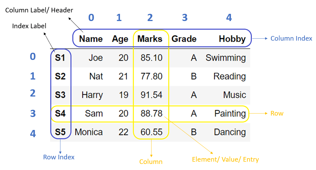
"Slicing" refers to subsetting, or extracting rows and columns from a data frame.
Here's the general syntax to identify dataframe positions in [ rows , columns ] where rows and columns can be either labels or indices.
loc allows us to subset data by row or column label. For example, if I would like to pull out the column 'sample_name', I would use the following command:
print(seq_info_input)

file_name    library_id     sample_name     body_length
s_1_1_CGATGT.fastq.gz    L23058    E1      7.5
s_1_1_TGACCA.fastq.gz    L23059    E2      7.7
s_1_1_TGACGG.fastq.gz    L23060    E3      8.9
..                ...              ..
s_1_1_ACAGTG.fastq.gz    L23078    E10     7.4

[10 rows x 4 columns]


print(seq_info_input.loc[:,"sample_name"])

sample_name
0    E1
1    E2
2    E3
..  ..
10  E10

[10 rows x 1 columns]
iloc allows us to subset rows and colums by index number. This is useful if we want to subset multiple rows or columns without typing index names.
print(seq_info_input.iloc[:3])

body_length
7.5
7.7
8.9
..
7.4
[10 rows, 1 column]


print(seq_info_input.iloc[2,:])

Name: file_name, Length: 336, dtype: object
file_name      s_1_1_TGACGG.fastq.gz
library_id                    L23059
sample_name                       E3
Name: 3, dtype: object
Note [[ ]] allows us to mention a list of columns.
# Return columns 0, 1, 3, 5, and 7
seq_info_input.iloc[:,[0,1,3,5,7]]


# Return rows 1 through 5 and columns 0, 1, 3, 5, and 7
seq_info_input.iloc[:5,[0,1,3,5,7]]
Here we'll take look at ordering our data by a particular column value, or multiple column values.
# Set ascending=True to reverse the order
seq_info_input.sort_values('sample_name', ascending=False)

# Sort by multiple columns in different directions
seq_info_input.sort_values(by=['sample_name', 'body_length'], ascending=[True, False])
Understanding how to subset your data using conditional operations is very, very useful. You'll often encounter situations where you want to filter your data on a certain set of parameters to reduce it to a more "meaningful" state.
# Subsetting on a single condition
seq_info_input.loc[(seq_info_input['body_length'] < 8 )]
In the example below we chain boolean operators together to achieve results that satisfy multiple conditions. You can make these statments complex as you'd like.
Note: Pandas uses the bitwise logical operators (see earlier lecture). A pipe symbol | represents or, and an ampersand symbol & represents and. The backslashes in code simply allow us to break up our statement at arbitrary points for readbility.
# Subsetting on multiple conditions.
seq_info_input[
    (seq_info_input['body_length'] < 7) | \
    (seq_info_input['sample_name'] == 'E3')]
What's actually going on here? The rows in the data frame are actually subsetted on a vector of True/False statements. That is, for every row for which the condition evaluates to True will be returned.
Subsetting might be the way you parse your RNA-seq results to a list of genes within a specific range of p-values and log fold changes, e.g., all p-values < 1e-15 and log fold changes > 1.2.
Lets look at a couple examples where we apply calculations to our data frame. First lets calculate some summary statistics. This can be a useful when viewing our results for the first time to get a handle on how our data is distributed.
# For this numerical data
data_df

   A   B    C   D   E
0  45  38   10  60  76
1  37  31   15  99  98
2  42  26   17  23  78
3  50  90  100  56  90


# Returning summary statistics for all columns
data_df.describe()

               A         B           C          D          E
count   4.000000   4.00000    4.000000   4.000000   4.000000
mean   43.500000  46.25000   35.500000  59.500000  85.500000
std     5.446712  29.57899   43.100657  31.118055  10.376255
min    37.000000  26.00000   10.000000  23.000000  76.000000
25%    40.750000  29.75000   13.750000  47.750000  77.500000
50%    43.500000  34.50000   16.000000  58.000000  84.000000
75%    46.250000  51.00000   37.750000  69.750000  92.000000
max    50.000000  90.00000  100.000000  99.000000  98.000000

# Returning summary statistics for a single column
data_df['A'].describe() # if you are working on a whole column
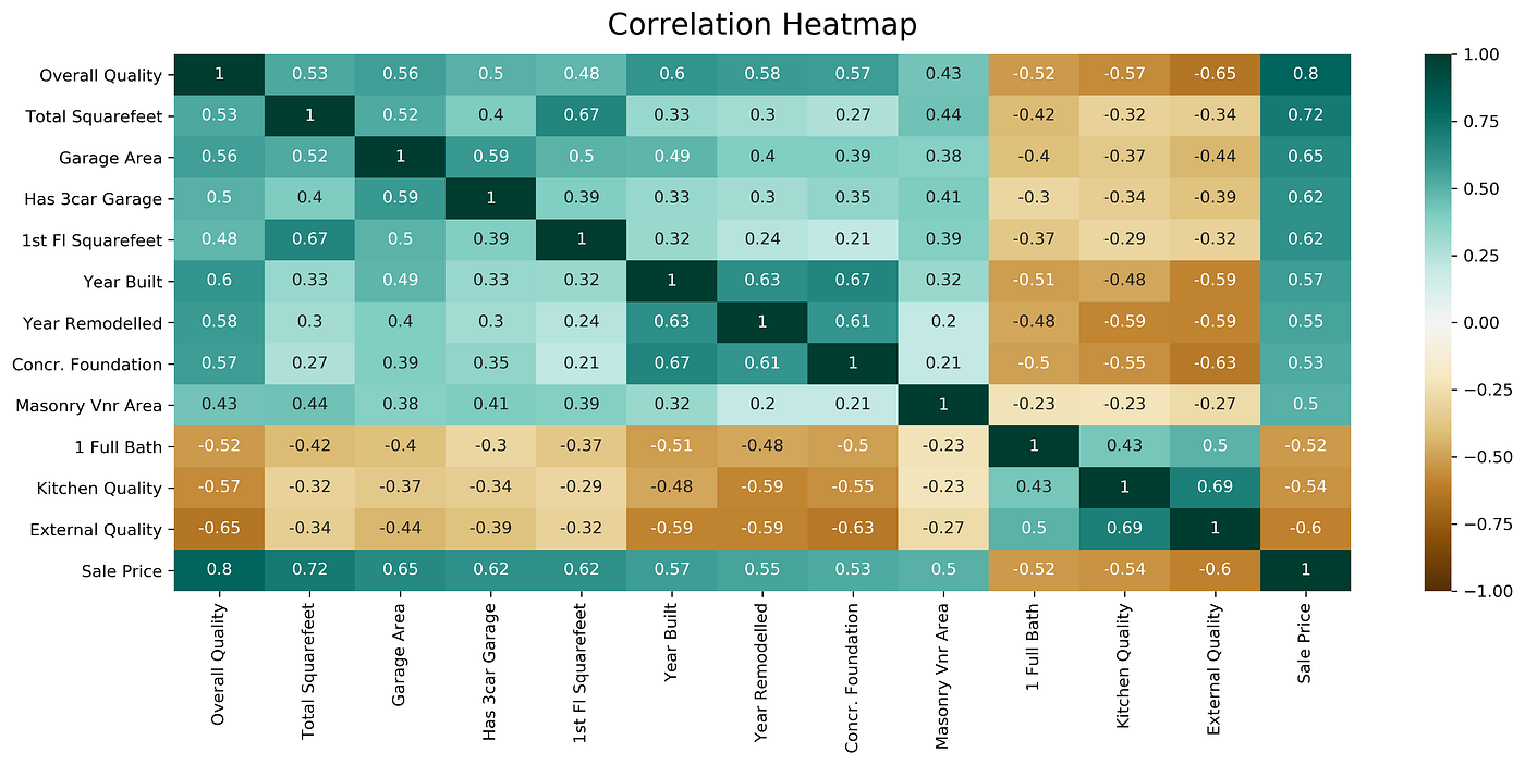
# Simply add the .corr() method to your dataframe subset
data_df.loc[:,['A','B']].corr()

          A         B
A  1.000000  0.830705
B  0.830705  1.000000
That summarizes our introduction to Pandas. As you can see, Pandas greatly simplifies the process of exploring and making calculations in data frames and matricies. Check out the link below for the official documentation.
Here's a few lines from a data file (fuelEfficiency.tsv)
| Mfr Name | Carline | Eng Displ | Cylinders | Transmission | CityMPG | HwyMPG | CombMPG | # Gears |
|---|---|---|---|---|---|---|---|---|
| aston martin | Vantage V8 | 4 | 8 | Auto(S8) | 18 | 25 | 21 | 8 |
| Volkswagen Group of | Chiron | 8 | 16 | Auto(AM-S7) | 9 | 14 | 11 | 7 |
| General Motors | CORVETTE | 6.2 | 8 | Auto(S8) | 12 | 20 | 15 | 8 |
| General Motors | CORVETTE | 6.2 | 8 | Auto(S8) | 15 | 25 | 18 | 8 |
| General Motors | CORVETTE | 6.2 | 8 | Auto(S8) | 14 | 23 | 17 | 8 |
It has 718 lines of data and a header line.
Let's examine the data in the file: data types, inconsistencies. What about trends in values?
We can use the python interpreter
>>> import pandas as pd
>>> import  matplotlib.pyplot as plt
>>> df = pd.read_csv('fuelEfficiency.tsv', sep='\t')
>>> df
                Mfr Name                 Carline  Eng Displ  Cylinders Transmission  CityMPG  HwyMPG  CombMPG  # Gears
0           aston martin              Vantage V8        4.0          8     Auto(S8)       18      25       21        8
1    Volkswagen Group of                  Chiron        8.0         16  Auto(AM-S7)        9      14       11        7
2         General Motors                CORVETTE        6.2          8     Auto(S8)       12      20       15        8
3         General Motors                CORVETTE        6.2          8     Auto(S8)       15      25       18        8
4         General Motors                CORVETTE        6.2          8     Auto(S8)       14      23       17        8
..                   ...                     ...        ...        ...          ...      ...     ...      ...      ...
713               Toyota             4RUNNER 4WD        4.0          6     Auto(S5)       17      20       18        5
714               Toyota  LAND CRUISER WAGON 4WD        5.7          8     Auto(S8)       13      18       15        8
715               Toyota             SEQUOIA 4WD        5.7          8     Auto(S6)       13      17       14        6
716                Volvo                XC90 AWD        2.0          4     Auto(S8)       19      26       22        8
717                Volvo                XC90 AWD        2.0          4     Auto(S8)       20      27       23        8
To get very useful summary statistics, use df.describe()
>>> df.describe()
        Eng Displ   Cylinders     CityMPG      HwyMPG     CombMPG     # Gears
count  718.000000  718.000000  718.000000  718.000000  718.000000  718.000000
mean     3.092061    5.493036   20.442897   27.760446   23.139276    7.147632
std      1.344572    1.752251    5.298504    5.607924    5.368443    1.507929
min      1.400000    3.000000    9.000000   14.000000   11.000000    1.000000
25%      2.000000    4.000000   17.000000   24.000000   19.000000    6.000000
50%      3.000000    6.000000   20.000000   27.000000   23.000000    7.000000
75%      3.600000    6.000000   23.000000   31.000000   26.000000    8.000000
max      8.000000   16.000000   57.000000   59.000000   58.000000   10.000000
We can make simple plots with pandas and matplotlib
We can show the distribution and range of a single set of data in a histogram.
Here are the bare bones, you can add/customize parameters yourself.
#!/usr/bin/env python3
import pandas as pd
import  matplotlib.pyplot as plt # we will use this plotting library

# read data into a pandas dataframe
df = pd.read_csv('fuelEfficiency.tsv', sep='\t')
fig,ax=plt.subplots(figsize=(6,6))
ax.hist(df['Cylinders'], bins=10)
# set title, axis labels
ax.set_xlabel('Number of cylinders')
ax.set_ylabel('Count')
ax.set_title('Vehicle fuel efficiency data')
#write histogram to a PNG graphics file
png_file = 'cylinders.hist.png'
fig.savefig(png_file)
print(f'Wrote {png_file}')
Here's the plot

These are great for looking at a relationship between two measurements or values.
#!/usr/bin/env python3
import pandas as pd
import  matplotlib.pyplot as plt # we will use this plotting library

fig,ax=plt.subplots(figsize=(6,6))
# set transparency with alpha and data point size with s
ax.scatter(df['Cylinders'],df['HwyMPG'], alpha = 0.5, s=2)
# set title, axis labels
ax.set_xlabel('Number of cylinders')
ax.set_ylabel('Highway Miles per Gallon')
ax.set_title('Vehicle fuel efficiency data')
#write histogram to a PNG graphics file
png_file = 'cylindersVShwyMPG.scatter.png'
fig.savefig(png_file)
print(f'Wrote {png_file}')
Here's the scatter plot. You can clearly see a relationship as well as variability in the data.

What's another good way to investigate a relationship between two sets of data?
That summarizes our introduction to Pandas. As you can see, Pandas greatly simplifies the process of exploring and making calculations in data frames and matricies. Check out the link below for the offical documentation.