PyHawkes implements a variety of Bayesian inference algorithms for discovering latent network structure given point process observations. Suppose you observe timestamps of Twitter messages, but you don't get to see how those users are connected to one another. You might infer that there is an unobserved connection from one user to another if the first user's activity tends to precede the second user's. This intuition is formalized by combining excitatory point processes (aka Hawkes processes) with random network models and performing Bayesian inference to discover the latent network.
We provide a number of classes for building and fitting such models.
Let's walk through a simple example
where we construct a discrete time model with three nodes, as in examples/discrete_demo.
The nodes are connected via an excitatory network such that each event increases
the likelihood of subsequent events on downstream nodes.
# Create a simple random network with K nodes a sparsity level of p
# Each event induces impulse responses of length dt_max on connected nodes
K = 3
p = 0.25
dt_max = 20
network_hypers = {"p": p, "allow_self_connections": False}
true_model = DiscreteTimeNetworkHawkesModelSpikeAndSlab(
    K=K, dt_max=dt_max, network_hypers=network_hypers)

# Generate T time bins of events from the the model
# S is the TxK event count matrix, R is the TxK rate matrix
S,R = true_model.generate(T=100)
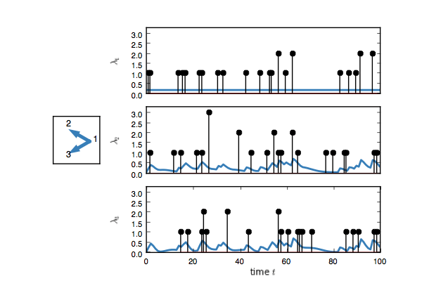
true_model.plot()
You should see something like this. Here, each event on node one adds
an impulse response on the rate of nodes two and three.

Now create a test model and try to infer the network given only the event counts.
# Create the test model, add the event count data, and plot
test_model = DiscreteTimeNetworkHawkesModelSpikeAndSlab(
    K=K, dt_max=dt_max, network_hypers=network_hypers)
test_model.add_data(S)
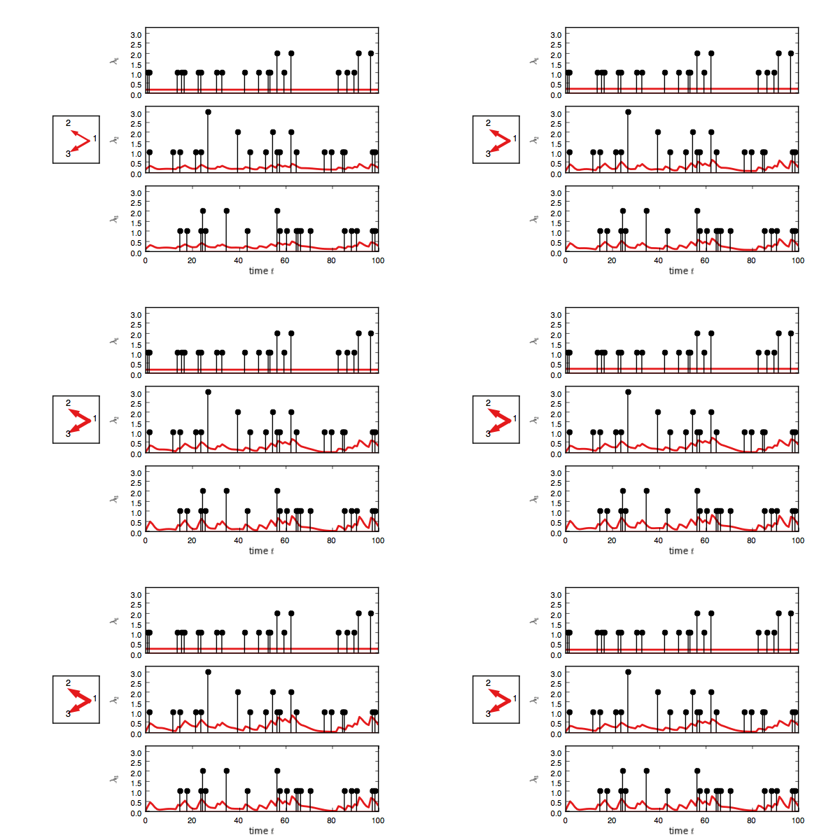
fig, handles = test_model.plot(color="#e41a1c")

# Run a Gibbs sampler
N_samples = 100
lps = []
for itr in range(N_samples):
    test_model.resample_model()
    lps.append(test_model.log_probability())

    # Update plots
    test_model.plot(handles=test_handles)
If you enable interactive plotting, you should see something like this.

In addition to Gibbs sampling, we have implemented maximum a posteriori (MAP) estimation,
mean field variational Bayesian inference, and stochastic variational inference. To
see how those methods can be used, look in examples/inference.
For a basic (but lower performance) installation run
pip install pyhawkes
To install from source run
git clone git@github.com:slinderman/pyhawkes.git
cd pyhawkes
pip install -e .
This will be rather slow, however, since the default version does not do any multi-threading. For advanced installation instructions to support multithreading, see MULTITHREADING.md.
This codebase is considerably cleaner than the old CUDA version, and is still quite fast with the Cython+OMP extensions and joblib for parallel sampling of the adjacency matrix.
Complete details of this work can be found in:
Linderman, Scott W. and Adams, Ryan P. Discovering Latent Network Structure in Point Process Data. International Conference on Machine Learning (ICML), 2014.
and
Linderman, Scott W., and Adams, Ryan P. Scalable Bayesian Inference for Excitatory Point Process Networks. arXiv preprint arXiv:1507.03228, 2015.