Deep Learning.md

[toc]

Deep Learning

Concept

• Neural Networks: At the core of deep learning are artificial neural networks, which consist of neurons (nodes) arranged in layers. A typical network comprises an input layer, multiple hidden layers, and an output layer.
• Learning Process: Neural networks learn by adjusting weights and biases within their neurons. This process is typically achieved through backpropagation, where the network adjusts its parameters based on the error of its predictions.
• Convolutional Neural Networks (CNNs): Specialized for processing structured grid data such as images, CNNs use convolutional layers to efficiently recognize spatial hierarchies in data.
• Recurrent Neural Networks (RNNs): Designed for sequential data (e.g., time series or text), RNNs have the unique feature of using their internal state (memory) to process sequences of inputs.
• Deep Learning Frameworks: Tools such as TensorFlow, PyTorch, and Keras simplify the development of deep learning models by providing libraries for creating and training neural networks.

Artificial Neural Networks

Neurons

• Inputs (x₁, x₂, ..., xn): Each neuron receives multiple inputs. These inputs can be raw data or outputs from other neurons.
• Weights (w₁, w₂, ..., wn): Each input is assigned a weight that represents its importance. The neural network learns by updating these weights.
• Bias (b): A bias term is added to the input-weight product, allowing the neuron to adjust the output along the activation function independently of its inputs.
• Activation Function: This function is applied to the weighted sum of the inputs plus the bias. It determines whether a neuron should be activated or not, influencing the neuron's output.
  • Sigmoid: Maps the input to a value between 0 and 1, useful for binary classification.
  • ReLU (Rectified Linear Unit): Outputs the input if it's positive; otherwise, it outputs zero. It's widely used for its computational efficiency and because it allows models to learn fast and effectively.
  • Tanh (Hyperbolic Tangent): Similar to the sigmoid but maps the input to values between -1 and 1, making it more suitable for certain types of normalized data.

Feedforward Network

• Input Layer: The first layer that receives the input signal to be processed. Each neuron in the input layer represents a feature of the input data.
• Hidden Layers: One or more layers that perform computations with signals received from the previous layer. Each neuron in these layers applies a weighted sum on its inputs, adds a bias, and then passes the result through an activation function.
• Output Layer: The final layer that produces the network's output. For classification tasks, this layer often uses a softmax activation function to output probabilities corresponding to each class.

Back Propagation

1. Initialize Weights: Randomly initialize the network's weights.
2. Perform a Forward Pass: Compute the output of the network and the loss.
3. Compute Gradients (Backward Pass): Use the chain rule to calculate the gradients of the loss function with respect to each weight.
4. Update Weights: Adjust the weights by a fraction (defined by the learning rate) of their gradients.
5. Repeat: Perform multiple iterations of forward and backward passes with weight updates until the network's performance is satisfactory or a certain number of iterations is reached.

$$ E_k=\frac{1}{2}\sum_j^l(\hat y_j^k-y_j^k)^2 $$

$$ \frac{\partial E_k}{\partial v_{ih}}=\sum_j^l\frac{\partial E_k}{\partial \hat y_j^k}\cdot \frac{\partial \hat y_j^k}{\partial \beta_j}\cdot \frac{\partial \beta_j}{\partial b_h}\cdot \frac{\partial b_h}{\partial \alpha_h}\cdot \frac{\partial \alpha_h}{\partial v_{ih}} $$

$$ \frac{\partial E_k}{\partial v_{ih}}=\sum_j^l(\hat y_j^k-y_j^k)\hat y_j^k(1-\hat y_j^k)w_{hj}b_h(1-b_h)x_i=\sum_j^l-g_jw_{hj}b_h(1-b_h)x_i $$

$$ \frac{\partial E_k}{\partial v_{ih}}=-b_h(1-b_h)\sum_j^lg_jw_{hj}x_i=-e_hx_i $$

Loss Functions

• Regression: Mean Squared Error (MSE) computes the average of the squares of the errors between the actual values ($y$) and the predicted values ($\hat{y}$). It's widely used in regression problems.

$$ MSE=\frac{1}{n}\sum_{i=1}^{n}(y_i-\hat{y_i})^2 $$

• Classification: Cross-entropy loss measures the performance of a classification model whose output is a probability value between 0 and 1. Often used in conjunction with the softmax function in the output layer for multiclass classification problems.

$$ Cross-Entropy=-\sum_{i=1}^n\sum_{c=1}^My_{ic}log(\hat{y_{ic}}) $$

Optimization

• Batch Gradient Descent: BGD computes the gradient of the loss function with respect to the parameters ((\theta)) for the entire training dataset.

  • Update Rule: $\theta = \theta - \eta \nabla_\theta J(\theta)$, where $\eta$ is the learning rate, and $J(\theta)$ is the cost function computed over the whole dataset.

  • Accuracy: Provides accurate updates as it considers the entire dataset.

  • Speed: Can be very slow with large datasets because it requires the entire dataset to be in memory and processes it all at once.

  • Convergence: Guaranteed to converge to the global minimum for convex error surfaces and to a local minimum for non-convex surfaces.

• Stochastic Gradient Descent: SGD updates the parameters for each training example one by one.

  • Update Rule: $\theta = \theta - \eta \nabla_\theta J(\theta; x^{(i)}, y^{(i)})$, where $x^{(i)}, y^{(i)}$ is a single training example.

  • Speed: Much faster per iteration than BGD because it updates the weights after each training example.

  • Noise: Updates are noisy (high variance), which can help escape local minima but may also prevent convergence to the exact minimum.

  • Convergence: The noisiness means it may never "settle" into a minimum but can oscillate in a small region, providing a good approximation.

• Mini-Batch Gradient Descent: MGD divides the training dataset into small batches and updates the model's parameters for each batch.

  • Update Rule: $\theta = \theta - \eta \nabla_\theta J(\theta; X_{\text{mini-batch}}, Y_{\text{mini-batch}})$, where $X_{\text{mini-batch}}, Y_{\text{mini-batch}}$ is a subset of the training data.

  • Balance: Strikes a balance between the efficiency of SGD and the stability of BGD.

  • Speed: Faster than BGD because it processes batches of the dataset at a time, which can be efficiently parallelized on modern hardware.

  • Convergence: More stable convergence than SGD but with some of the benefits of noise, helping to escape local minima.

• Gradient descent with Momentum: Accelerates SGD in the relevant direction and dampens oscillations, improving convergence speed

$$ v_{dW^{[l]}} = \beta v_{dW^{[l]}} + (1 - \beta) dW^{[l]} $$

$$ v_{db^{[l]}} = \beta v_{db^{[l]}} + (1 - \beta) db^{[l]} $$

$$ W^{[l]} := W^{[l]} - \alpha v_{dW^{[l]}} $$

$$ b^{[l]} := b^{[l]} - \alpha v_{db^{[l]}} $$

• Adagrad (Adaptive Gradient Problem): Adapts the learning rate to the parameters, performing smaller updates for parameters associated with frequently occurring features, and larger updates for parameters associated with infrequent features.

$$ s_{dw} = s_{dw} + (dw)^2 $$

$$ s_{db} = s_{db} + (db)^2 $$

$$ w := w - \frac{\alpha}{\sqrt{s_{dw} + \epsilon}}dw $$

$$ b := b - \frac{\alpha}{\sqrt{s_{db} + \epsilon}}db $$

• **RMSprop (Root Mean Square Propagation): **Addresses AdaGrad's radically diminishing learning rates by using a moving average of squared gradients to normalize the gradient. This ensures the learning rate doesn't decrease too quickly.

$$ s_{dw} = \beta s_{dw} + (1 - \beta)(dw)^2 $$

$$ s_{db} = \beta s_{db} + (1 - \beta)(db)^2 $$

$$ w := w - \frac{\alpha}{\sqrt{s_{dw} + \epsilon}}dw $$

$$ b := b - \frac{\alpha}{\sqrt{s_{db} + \epsilon}}db $$

• **Adam (Adaptive Moment Estimation): **Combines ideas from RMSprop and SGD with momentum by keeping an exponentially decaying average of past gradients and squared gradients. It adjusts the learning rate for each weight individually.

$$ v_{dW} = \beta_1 v_{dW} + (1 - \beta_1) dW $$

$$ v_{db} = \beta_1 v_{db} + (1 - \beta_1) db $$

$$ s_{dW} = \beta_2 s_{dW} + (1 - \beta_2) {(dW)}^2 $$

$$ s_{db} = \beta_2 s_{db} + (1 - \beta_2) {(db)}^2 $$

$$ v^{corrected}{dW} = \frac{v{dW}}{1-{\beta_1}^t} $$

$$ v^{corrected}{db} = \frac{v{db}}{1-{\beta_1}^t} $$

$$ s^{corrected}{dW} = \frac{s{dW}}{1-{\beta_2}^t} $$

$$ s^{corrected}{db} = \frac{s{db}}{1-{\beta_2}^t} $$

$$ W := W - \frac{\alpha}{{\sqrt{s^{corrected}{dW}} + \epsilon}}v^{corrected}{dW} $$

Regularization

• Dropout: Dropout randomly "drops" (i.e., temporarily removes) a proportion of neurons in the network during training at each iteration, preventing them from participating in forward pass and backpropagation. This randomness forces the network to learn more robust features that are useful in conjunction with many different random subsets of the other neurons.

• Batch Normalization: Batch normalization standardizes the inputs to a layer for each mini-batch. This stabilizes the learning process and dramatically reduces the number of training epochs required to train deep networks.

• Early Stopping: Early stopping involves monitoring the network's performance on a validation set and stopping training when performance deteriorates, as evidenced by an increase in validation set error.

• **Data Augmentation: **Data augmentation artificially increases the size and variability of the training dataset by applying random transformations (e.g., rotation, scaling, cropping, flipping, or changing the lighting conditions) to the existing training samples. This helps the model generalize better to new, unseen data.

Convolutional Neural Networks

Architecture

• **Convolutional Layer: **The convolutional layer is the core building block of a Convolutional Neural Network (CNN). Its primary function is to detect patterns such as edges, colors, textures, and complex shapes within the input images.
  • Filters/Kernels: A convolutional layer consists of several filters (or kernels) that are small but extend through the full depth of the input volume. For instance, in an RGB image, a filter would have a depth of 3, corresponding to the three color channels.
  • Convolution Operation: As a filter is slid (or convolved) across the input image, it performs element-wise multiplication with the part of the image it covers and sums up these multiplications. This process is repeated across the entire image, producing a feature map for each filter.
  • Strides: The stride determines how much the filter moves across the image. A stride of 1 moves the filter one pixel at a time, while a larger stride moves the filter more pixels, reducing the size of the output feature map.
  • Padding: To control the size of the feature maps, padding can be added to the input image. Zero-padding pads the input image with zeros around the border, allowing for control over the spatial size of the output volumes.
  • Activation Function: Typically, after a convolution operation, an activation function like ReLU (Rectified Linear Unit) is applied to introduce non-linearity, enabling the network to learn complex patterns.

• **Pooling Layer: **Pooling layers follow convolutional layers and are used to reduce the spatial dimensions (width and height) of the input volume for the next convolutional layer. This reduction in dimensionality means less computation and memory usage, as well as less chance of overfitting.
  • Max Pooling: The most common form of pooling, where the maximum element is selected from the region of the feature map covered by the filter, typically of size 2x2.
  • Average Pooling: Calculates the average of the elements in the region of the feature map covered by the filter.
  • Global Pooling: Reduces each feature map to a single value by taking the average or maximum of all elements in the feature map.

LeNet

• Input Layer: The original LeNet-5 architecture accepts a 32×32 pixel grayscale image as input. This size is chosen to ensure that the handwritten digits fit well within the field of view of the convolutional layers.
• Convolutional Layers: The network uses convolutional layers with small filter sizes (e.g., 5×5) to learn spatial hierarchies of features from the input image. These layers apply a set of learnable filters to the input, creating a series of feature maps.
• Activation Functions: After each convolutional layer, an activation function, typically the sigmoid or tanh in the original LeNet-5 model, is applied to introduce non-linearity into the model, allowing it to learn more complex patterns.
• Pooling (Subsampling) Layers: LeNet uses average pooling layers (also known as subsampling) to reduce the spatial dimensions of the feature maps, thereby reducing the computational complexity and helping to make the representation more invariant to small translations of the input.
• Fully Connected Layers: Towards the end of the network, fully connected layers are used to perform high-level reasoning based on the features extracted by the convolutional and pooling layers. The final layer uses a softmax activation function to output a probability distribution over the target classes.
• Output Layer: Produces the final classification output, with each neuron corresponding to a class label (e.g., digits 0-9 in the case of handwritten digit recognition).

AlexNet

• **Convolutional Layers: **These layers perform convolution operations, applying filters (or kernels) to the input images to extract features such as edges, textures, and other patterns. The filters are learned during the training process.

• **ReLU (Rectified Linear Unit) Layers: **Follows directly after each convolutional layer and introduces non-linearity into the model, allowing it to learn complex patterns.

• **Pooling (Max Pooling) Layers: **These layers are used to reduce the spatial dimensions (width and height) of the input volume for the next convolutional layer. It helps to decrease the computational load, memory usage, and also helps to prevent overfitting.

• **Normalization Layers (Local Response Normalization): ** This layer enhances the computed activity of neurons that are more strongly activated while suppressing weaker activations, making the network less sensitive to high-frequency features and improving generalization.

• **Fully Connected Layers: ** These layers are used to flatten the high-level features learned by convolutional layers and combine them to form a model. The output from the last fully connected layer is fed to a softmax classifier to obtain the final classification probabilities for each class.

• **Dropout Layers: **Introduced just before the first and the second fully connected layers, dropout is a regularization technique to prevent overfitting in the neural network.

• **Softmax Output Layer: **The final layer in AlexNet is a softmax layer that outputs a distribution over the 1000 class labels, converting the scores into probabilities.

VGG

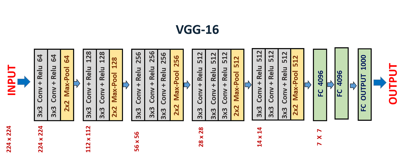
• Convolutional Layers: VGG networks use 3x3 convolutional filters with a stride of 1 pixel; this small receptive field allows capturing fine details in the image. The convolutional layers are arranged in blocks, with each block followed by a max-pooling layer for spatial downsampling.
• Depth: The networks are notably deep, with VGG-16 and VGG-19 having 16 and 19 layers respectively. This depth is crucial for learning a hierarchy of features at different scales and complexities.
• Fully Connected Layers: Following several blocks of convolutional and max-pooling layers, VGG networks have three fully connected layers. The first two have 4096 channels each, and the third performs classification, having as many channels as there are classes in the dataset (e.g., 1000 for ImageNet).
• ReLU Activation: The ReLU (Rectified Linear Unit) activation function is applied after each convolutional layer, introducing non-linearity into the model without affecting the receptive fields of the convolution layers.
• Fixed Input Size: VGG networks are trained with a fixed input size of 224x224 RGB images, which means that all images need to be resized to this dimension before being fed into the network.
• Pre-training: VGG networks were pre-trained on the ImageNet dataset, which contains over a million images categorized into 1000 classes. This pre-training helps in transferring learned features to other visual recognition tasks with less data.

ResNet

• Residual Blocks: The core idea behind ResNet is its use of residual blocks. These blocks have a shortcut connection that skips one or more layers and performs identity mapping, adding the input of the block to its output. This design encourages the network to learn residual functions with reference to the layer inputs, making it easier to train deeper networks.
• Deep Architectures: ResNet architectures come in various depths, with ResNet-18, ResNet-34, ResNet-50, ResNet-101, and ResNet-152 being some of the most popular configurations. The number denotes the total layers in the architecture. The deeper versions of ResNet, like ResNet-50 and beyond, use "bottleneck" layers with 1x1, 3x3, and 1x1 convolutional layers in their residual blocks to increase depth without a significant increase in computational complexity.
• Batch Normalization: ResNet applies batch normalization after every convolutional layer. This technique normalizes the output of a previous activation layer by subtracting the batch mean and dividing by the batch standard deviation, which helps in speeding up training and reduces the sensitivity to network initialization.
• Global Average Pooling: Instead of using fully connected layers at the end of the network, ResNet employs global average pooling to reduce the dimensions of the feature maps to the number of classes, which significantly decreases the number of parameters and helps to prevent overfitting.

Recurrent Neural Networks

RNN

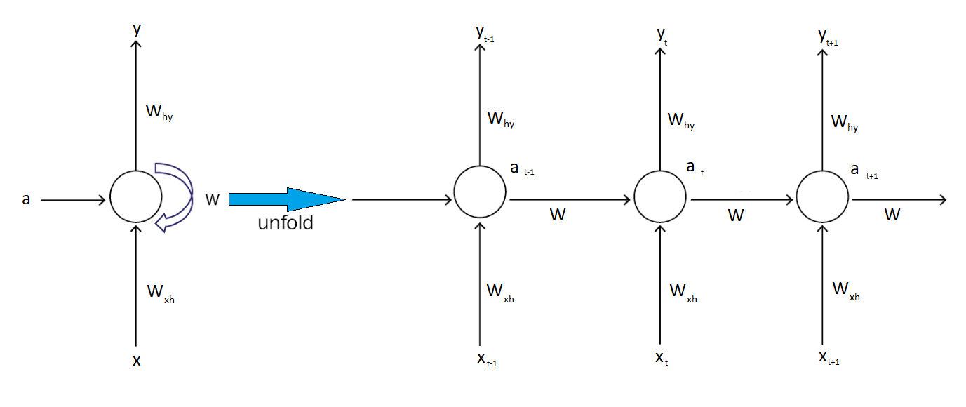
• Sequence Processing: Unlike feedforward neural networks, RNNs are designed to work with sequences of data, where the order and context of the input elements are crucial for making accurate predictions or generating outputs.
• Shared Weights: In an RNN, the same weights are applied across all time steps during the forward and backward passes, which significantly reduces the number of parameters that need to be learned, regardless of the sequence length.
• Memory: RNNs have a form of memory that captures information about what has been calculated so far. The output at each time step depends not just on the current input but also on a hidden state, which represents the information learned from prior inputs.
• Variable Length Inputs and Outputs: RNNs can handle inputs and outputs of varying lengths, making them versatile for a wide range of tasks such as generating variable-length text or processing audio clips of different durations.

LSTM

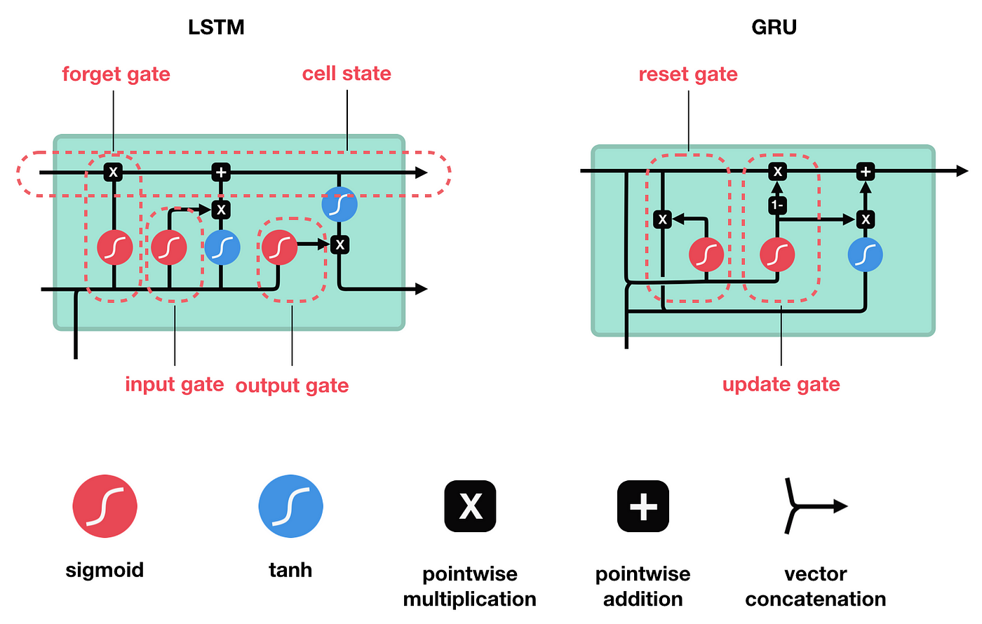
• Forget Gate: Decides what information is irrelevant and should be thrown away from the cell state.

$$ f_t = \sigma(W_f \cdot [h_{t-1}, x_t] + b_f) $$

• Input Gate: Updates the cell state with new information from the current input.

$$ i_t = \sigma(W_i \cdot [h_{t-1}, x_t] + b_i) $$

$$ \tilde{C}t = \tanh(W_C \cdot [h{t-1}, x_t] + b_C) $$

• **Cell State: **

$$ C_t = f_t * C_{t-1} + i_t * \tilde{C}_t $$

• Output Gate: Determines what the next hidden state should be, which is used for predictions and passed to the next time step.

$$ o_t = \sigma(W_o \cdot [h_{t-1}, x_t] + b_o) $$

$$ h_t = o_t * \tanh(C_t) $$

GRU

• Update Gate: Helps the model to determine the extent to which the new state is just the old state and to what extent the new state is influenced by the current input.

$$ z_t = \sigma(W_z \cdot [h_{t-1}, x_t] + b_z) $$

• Reset Gate: Allows the model to decide how much of the past information to forget.

$$ r_t = \sigma(W_r \cdot [h_{t-1}, x_t] + b_r) $$

• Hidden State:

$$ \tilde{h}t = \tanh(W \cdot [r_t * h{t-1}, x_t] + b) $$

$$ h_t = (1 - z_t) * h_{t-1} + z_t * \tilde{h}_t $$

Sequence to Sequence

• Encoder: The encoder processes the input sequence one element at a time and transforms it into a fixed-sized context vector. Decoder

• Decoder: The decoder is tasked with generating the output sequence, element by element, using the context vector as its initial state. It is also typically an RNN that is trained to predict the next element of the output sequence, given the previous elements and the context vector.

Generative Models

VAE

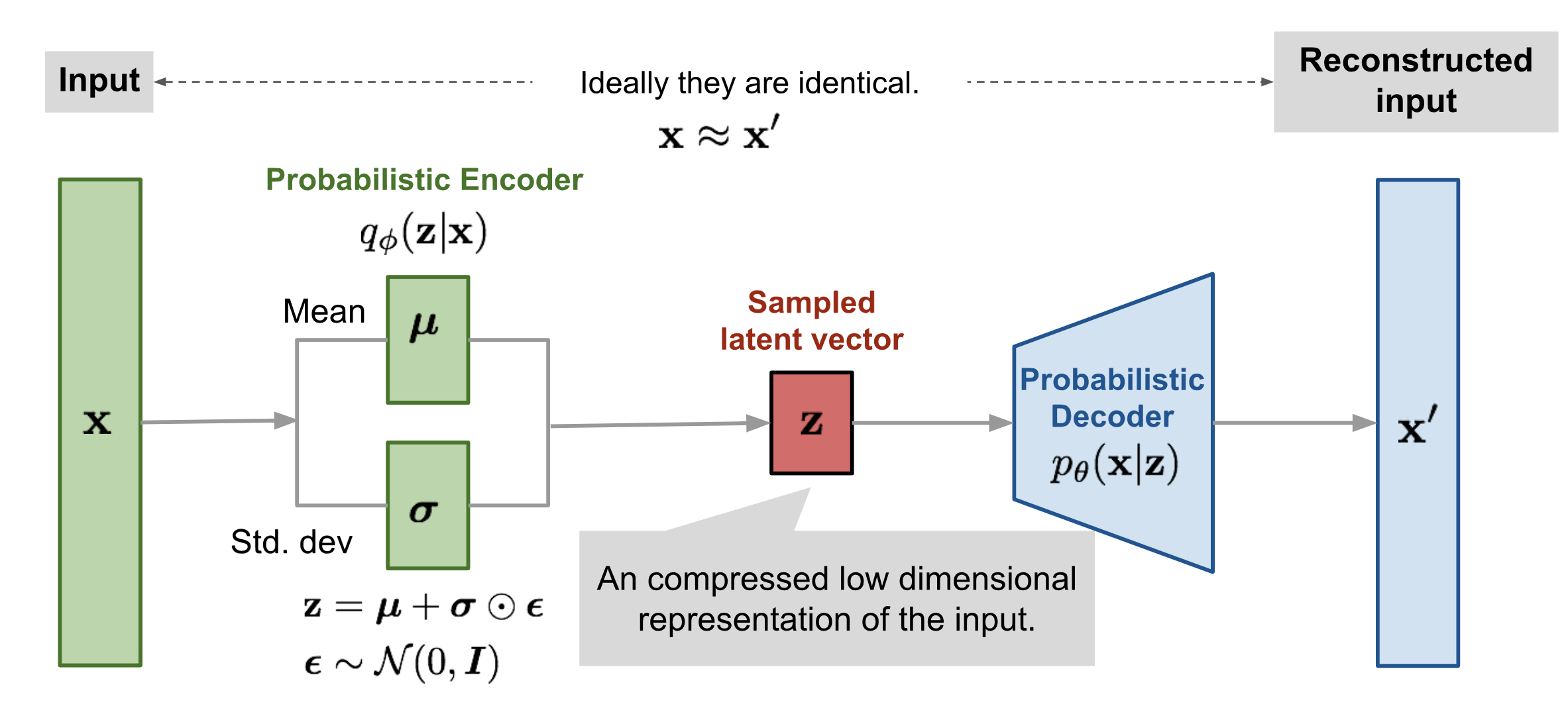
• Encoding: The encoder part of a VAE takes an input x and encodes it into a latent representation z*. However, instead of encoding x to a single point, the encoder outputs parameters (mean μ and variance 2σ2) of a probability distribution in the latent space.
• Sampling: A point z* is sampled from the distribution defined by μ* and 2σ2. This sampling introduces randomness into the model, which is crucial for the generative process.
• Decoding: The decoder takes the sampled latent point z* and tries to reconstruct the original input x.
• Loss Function: The loss function of a VAE is composed of two terms: a reconstruction loss (e.g., Mean Squared Error) that forces the decoded samples to match the original inputs, and a regularization term (Kullback-Leibler divergence) that pushes the latent space distributions to be as close as possible to a prior distribution, typically a standard normal distribution.

GAN

• Generator: The generator network takes random noise as input and generates data (like images) that resemble the training data. The goal of the generator is to produce data so realistic that the discriminator cannot distinguish it from real data.

• Discriminator: The discriminator network takes real data from the training set and fake data from the generator as input and tries to classify them as real or fake. Its goal is to accurately identify whether the input data is coming from the training dataset or was created by the generator.

• **Training: **The training of GANs involves a competitive process where the generator and discriminator are trained simultaneously. The generator aims to maximize the probability of the discriminator making a mistake, while the discriminator aims to minimize this probability. This process can be described as a min-max game with the following objective function:

$$ \min_{G} \max_{D} V(D, G) = \mathbb{E}{x \sim p{\text{data}}(x)}[\log D(x)] + \mathbb{E}{z \sim p{z}(z)}[\log(1 - D(G(z)))] $$