-
Notifications
You must be signed in to change notification settings - Fork 0
Overview of the Machine Learning Models
We first handle the missing data by taking away unavailable rows. Afterwards, we format our table by applying an SQL transformation. Feature picking is also done in this stage.
Then, we pass the whole dataframe into a Python script, which searches for recent history data and put it into the current row (e.g. from a schema of [DateTime, Pollution_Level] to [DateTime, Previous_Hour_Pollution_Level, Current_Pollution_Level]). This model is highly customizable where the number and the offset of history data lookup, reflecting the changes to the input table, number of location can be easily specified in the beginning. The column names are also handled properly such that they are legible.
We finalize the data processing by sorting them based on time and then the location by applying an SQL transformation.
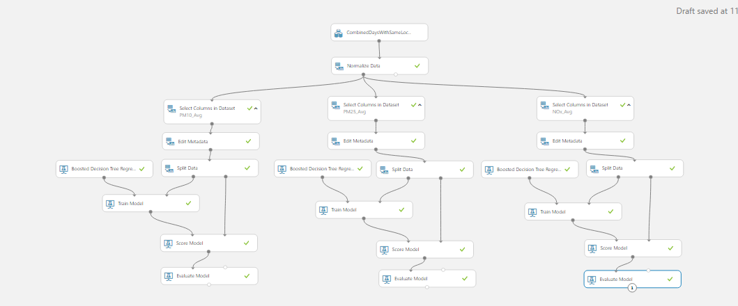
The data is first nomralized and then passed into three training pipelines, each corresponds to one of the pollutants. The following parts are typical modules used for training models: picking the labelled column, passing the splitting the dataset into training set and testing set, training the model and evaluating the model.
After training several models and evaluating their fitness, the best models are chosen and used in the web service. Here, we require the input from user having the same schema as our training dataset. Then, follow the same flow what we did in the training stage, except for swapping the training modules to the trained models. We then combine the predictions of all the three pollutants and then apply the denormalization and output the reults.
In this stage, we test the fitness of the model if it is used for predicting further into the future using the predictions by itself. The bootstrpping is done by first getting predictions and then put back into the same model for further prediction.
In the Day model training, we apply aggregate queries in in the data processing stage, such that average over the whole day can be obtained. Other data flows are similar to that of the Hour model.
A large part of this module originates from the “Retail Forecasting Template” Experiment by AzureML Team for Microsoft. Further details can be found on the Cortana Intelligence Gallery: https://gallery.cortanaintelligence.com/Collection/Retail-Forecasting-Template-1
We first fix the format of input data to match the imported R library. A particular period is then selected for training and for testing. Afterwards, missing rows are inserted with NA value such that we can have a contiguous block of data.
We then pass the data into training two time series models: “Seasonal Trend Decomposition using Loess (STL) + Exponential Smoothing (ETS)” and “Seasonal Trend Decomposition using Loess + AutoRegressive Integrated Moving Average (ARIMA)”.
The predicted results are compared to the observed data and error rates are evaluated.


