pipemesh

These tools use the GMSH-SDK (or GMSH-API), available here.

The documentation for pipemesh can be found here.

Requirements:

• libgmsh.so, libgmsh.so.4.3, libgmsh.so.4.3.0 (or higher) from the GMSH SDK. Download the SDK and navigate to the lib/ folder to find these, or use the versions hosted in this repository.
• SciPy (and NumPy, installed with SciPy).

pipemesh is currently only supported on Linux systems (e.g. Ubuntu 16, 18).

Installation

$python3 -m pip install --user pipemesh

Once completed, navigate to site-packages/pipemesh of the python installation used. Place the files libgmsh.so, libgmsh.so.4.3 and libgmsh.so.4.3.0 in this folder.

A virtual environment can be useful to locate the site-packages directory more easily.

# If you don't have venv
$sudo apt-get install python3-venv

$mkdir virtual_env # Name of your virtual environment
$python3 -m venv virtual_env
$source virtual_env/bin/activate
$python3 -m pip install –upgrade pip
$python3 -m pip install --user scipy
$python3 -m pip install --user pipemesh

Then simply place the libgmsh files into virtual_env/lib/site-packages/pipemesh/. Ensure to use the virtual environment every time you need to use pipemesh.

If you really don't want to use pip to install, clone the repository, and add acse-9.../pipemesh/ to PATH so python can find it.

pipes.py

Once installed, scripts to generate pipe and pipe network meshes can be created. A script is started by creating the Network object:

from pipemesh import pipes
network = pipes.Network(1, 0.3, [1,0,0], 0.1)

Then added to using one of the following commands:

network.add_cylinder(1, 0.1, out_number=1)
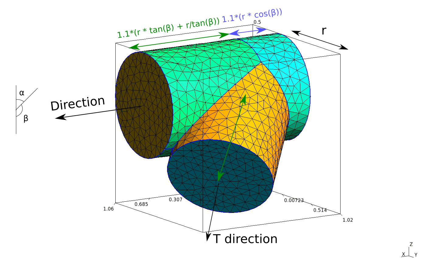
network.add_t_junction([-1,-1,0], 0.05)
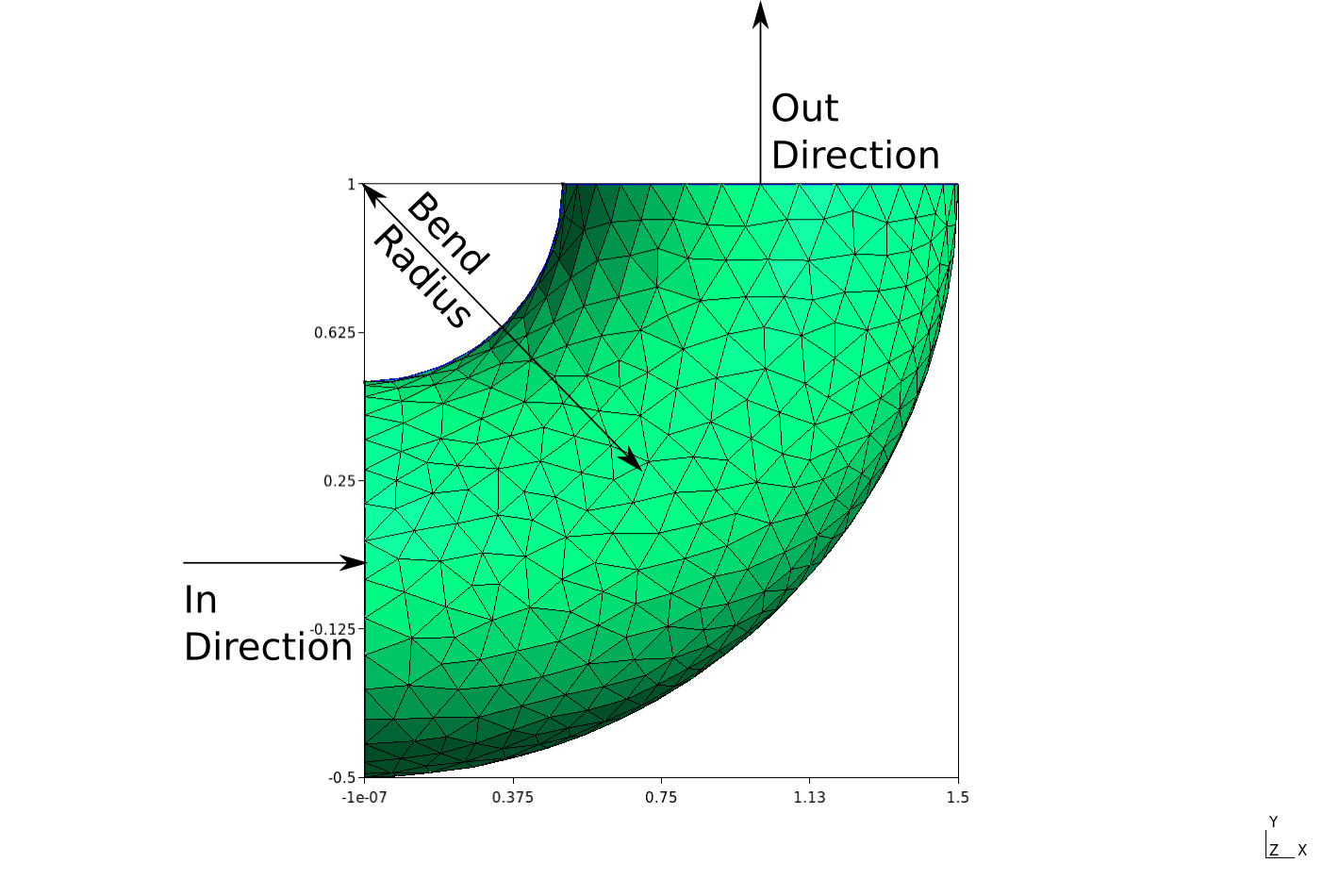
network.add_curve([0,1,0], 0.5, 0.05)
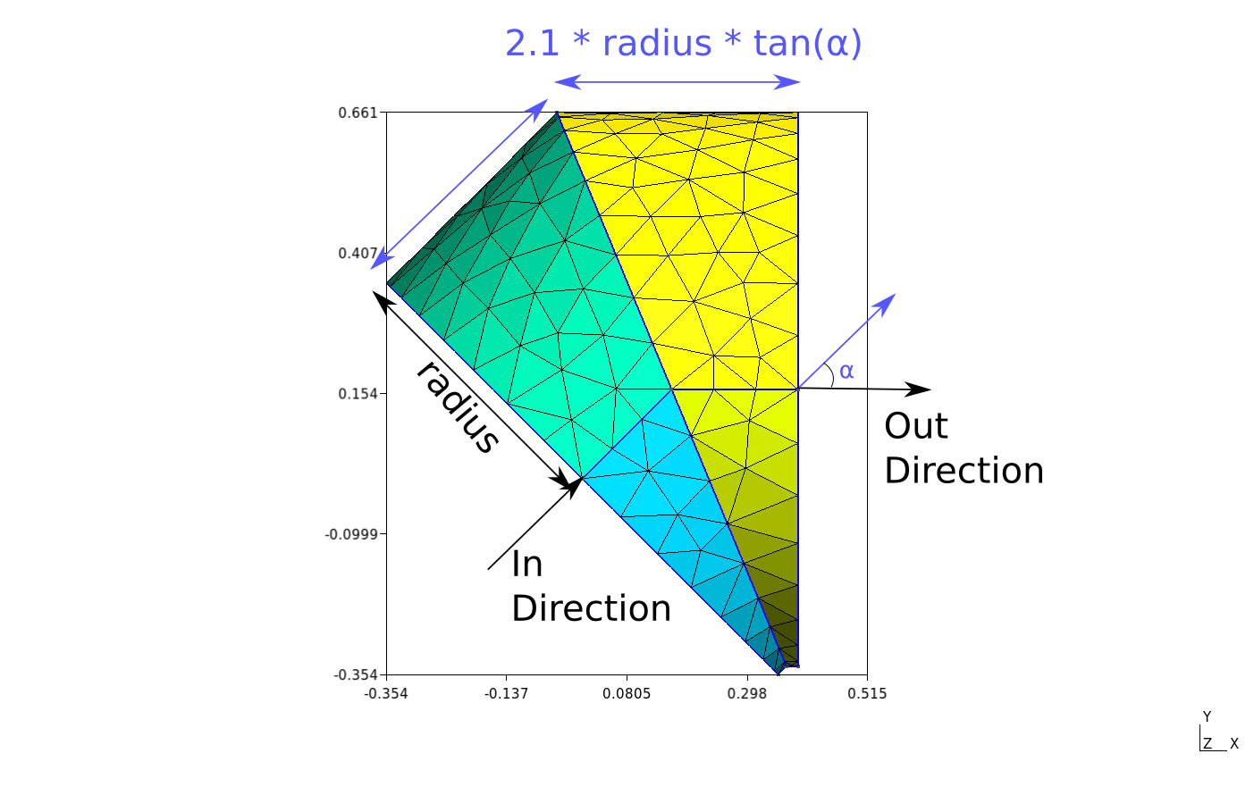
network.add_mitered([0, 1, 0], 0.05, out_number=2)

Where out_number specifies which outlet of the pipe the piece will be added to. For more information on each function, please visit the documentation linked above.

Examples:

• Chicane with mitered bends:

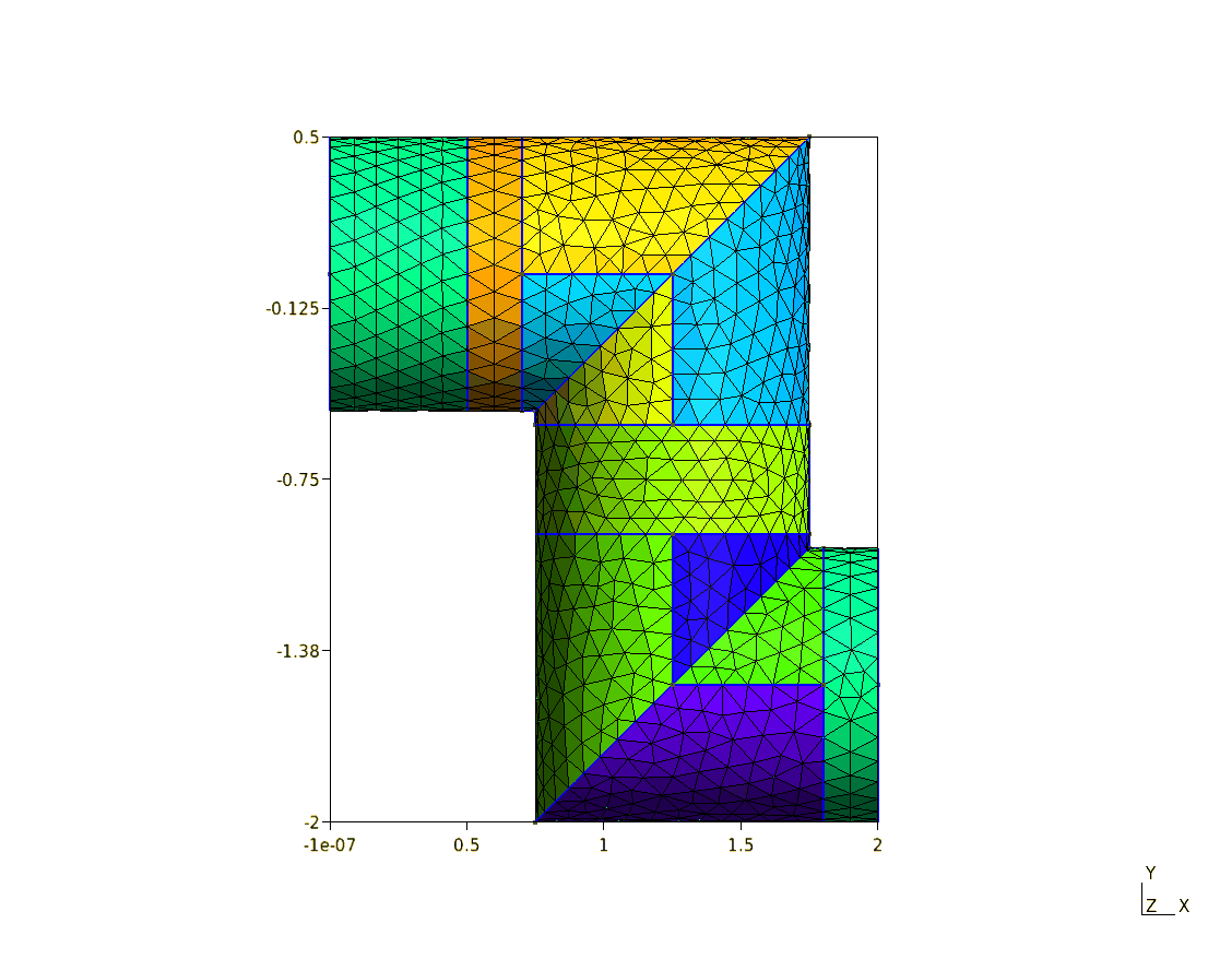
network = pipes.Network(1, 0.3, [1,0,0], 0.1)
network.add_cylinder(1, 0.1)
network.add_mitered([0,1,0], 0.1)
network.add_cylinder(1, 0.1)
network.add_mitered([1,0,0], 0.1)
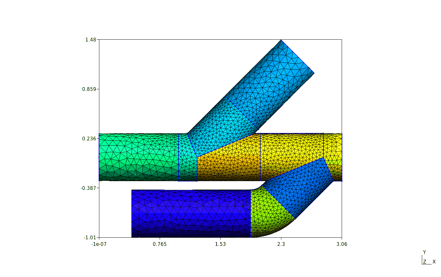
network.add_cylinder(1, 0.1)

• Pipe with two junctions:

network.add_t_junction([-1,1,0], 0.05)
network.add_t_junction([-1,-1,0], 0.05)
network.add_cylinder(1, 0.1, out_number=2)
network.add_curve([-1,0,0], 0.5, 0.05, out_number=3)
network.add_cylinder(1.5, 0.1, out_number=3)

Once the Network is complete, you can fuse the objects together and create physical surfaces and volumes, and set the local mesh sizes. Information can be obtained and written to file. This is all done with one call.

network.generate(filename="example", binary=False, write_info=False, mesh_format="msh2", write_xml=False run_gui=False)

Which will write the file "example.msh", as a msh2 binary file.

Network has get_phys_ids methods, which can be used with AutoMPML.

AutoMPML

The file auto_mpml.py contains the class AutoMPML. This edits a basic pipe flow simulation .mpml file used with IC-FERST by inputting the user values in the right places. This isn't actually automatic, but can save time by not editing mpml files with Diamond. Options that can be changed are relevant to conducting a pipe flow investigation with IC-FERST.

Example:

from pipemesh import pipes
from pipemesh.icferst import auto_mpml

# Generate a network
network = pipes.Network(0.1, 0.3, [0, 0, -1], 0.1)
network.add_t_junction([1, 0, 1], 0.1)
network.generate(filename="pipe", binary=True, write_info=True, write_xml=True, run_gui=False)

# Get physical ids of inlets and outlets
entry_phys_ids = network.get_inlet_outlet_phys_ids()
# Get physical ids of cylinder surfaces
cyl_phys_ids = network.get_cyl_phys_ids()
# Select the inlet and the first outlet as inlets
inlets = entry_phys_ids[:2]
# Select the remainding inlet/outlets as outlets
outlets = entry_phys_ids[2:]

# Get velocity vectors for velocity magnitude 0.02
vel = 0.02
inlet_velocities = network.get_velocities_vel_mag(inlets, vel, 1000, 1e-3)

# Create options object
options = auto_mpml.AutoMPML()
# Change various options (the defaults are fairly sensible)
options.set_all(sim_name="junction_flow_test_case",
                msh_file="src/pipe",
                dump_ids=entry_phys_ids,
                density=1000,
                inlet_phys_ids=inlets, inlet_velocities=inlet_velocities,
                outlet_phys_ids=outlets,
                cyl_phys_ids=cyl_phys_ids,
                max_no_nodes=10000,
                min_mesh_size=0.2,
                finish_time=1.0,
                t_adapt_delay=0.5
                )
# Write mpml file - extension not needed.
options.write_mpml("generated_mpml")

As the options can be set in python, this means that multiple simulations can be set up, with for example, varying reynolds numbers or varying input surfaces. For full information on what settings can be changed, visit the documentation.

pieces.py

Contains classes (and some useful functions for said classes) which represent cylindrical GMSH objects. The classes store information of the object, such as the centre and direction of its faces, as well as functions to update the information when transformations are applied to them. This makes the information a little easier to access than using just the GMSH API. To use these individually start your file with:

from pipemesh import pieces, gmsh
model = gmsh.model
mesh = model.mesh
gmsh.initialize()
gmsh.option.setNumber("Mesh.CharacteristicLengthMax", 0.1)  # max mesh length
model.add("Example")  # optional, add a model name.

The available pieces to put in are:

• Cylinder

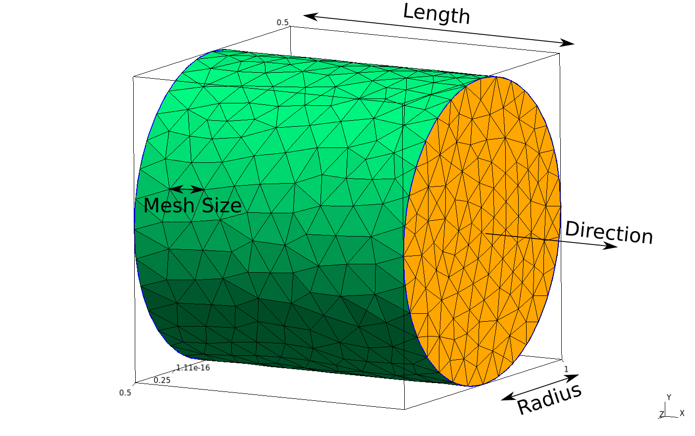
piece = pieces.Cylinder(1, 0.5, [1,0,0], 0.1)
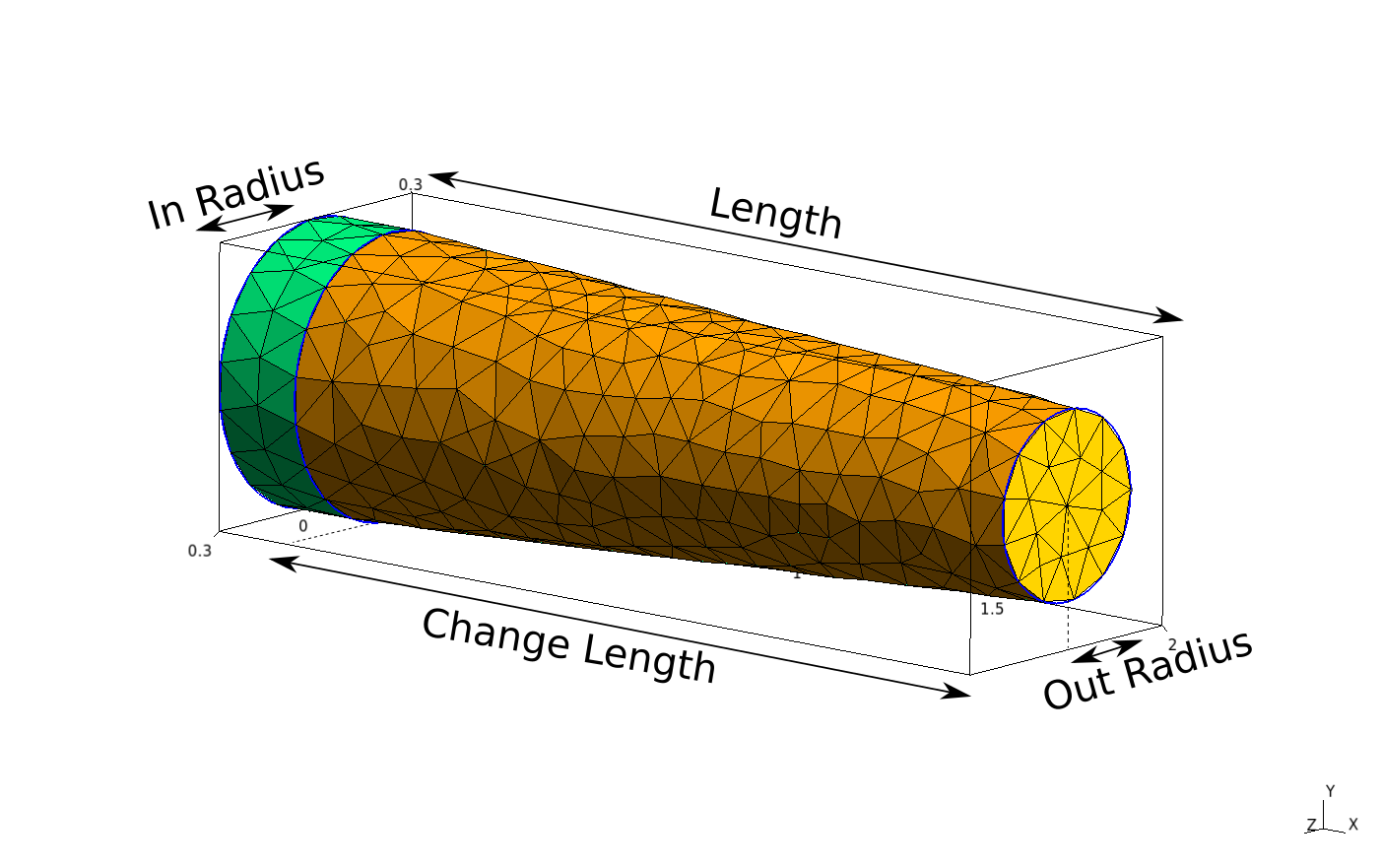
# Length, radius, direction, mesh size

• Cylinder with changing radius

piece = pieces.ChangeRadius(2, 1.8, 0.3, 0.2, [1 ,0, 0], 0.1)
# length, change length, start radius, end radius, direction, mesh size

• Smooth bends

piece = pieces.Curve(0.5, [1,0,-1], [0,1,0], 1, 0.2)
# radius of cylinder, in direction, out direction, bend radius, mesh size

• Mitered bends

piece = pieces.Mitered(0.5, [0, 1, 0], [1, 0, 0], 0.2)
# radius of cylinder, in direction, out direction, mesh size

• T Junctions

piece = pieces.TJunction(0.5, [1, 0, 0], [1, 1, -1], 0.1)
# radius, direction, t direction, mesh size

The mesh can be created and saved using:

mesh.generate(3)
gmsh.option.setNumber("Mesh.Binary", 1)  # 1 for binary, 0 for ASCII
gmsh.write(filename.msh)  # .msh2 for legacy format

To view the mesh in the GMSH GUI, call

gmsh.fltk.run()

To finish, and end use of gmsh, call

gmsh.finalize()