Machine Learning Notes

What is machine learning?

2 Linear Models 1: Hyperplanes, Random Search, Gradient Descent (MLVU2019)

Hyperplanes

• dot product
• 2d linear function

Random Search

• optimization random search: it test if the next random point is better than the previous one and if yes it switch, from probability q now and then we test if there is another better solution and check if there is a global minimum or we already reach it.
  • if loss(p) < loss(p')
    • p <- p'
  • else:
    • probability q: p <- p'
• compute only loss function
• require many interaction
• work with trees discrete models
• can be parallelized

Gradient descent

Definitions

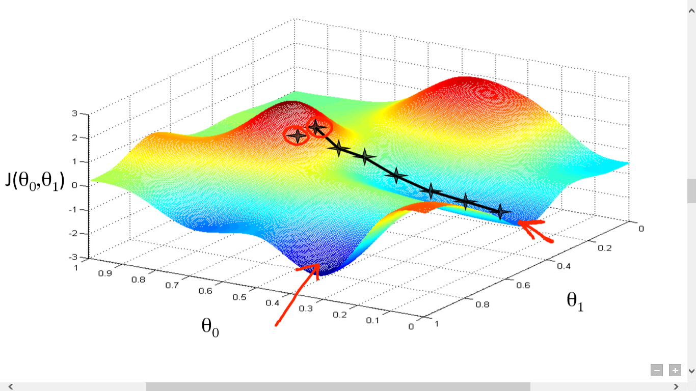
Gradient Descent requires a cost function(there are many types of cost functions). We need this cost function because we want to minimize it. Minimizing any function means finding the deepest valley in that function. Keep in mind that, the cost function is used to monitor the error in predictions of an ML model. So minimizing this, basically means getting to the lowest error value possible or increasing the accuracy of the model. In short, We increase the accuracy by iterating over a training data set while tweaking the parameters(the weights and biases) of our model.

So, the whole point of GD is to minimize the cost function.

• Gradient descent computes the direction of steepest descent.
• Accuracy is a bad loss function in gradient descent, becasue gradient descent makes the gradient zero almost everywhere.
• no escape local minima

---

4 Methodology 2: Data cleaning, Principal Component Analysis, Eigenfaces (MLVU2019)

Principal Component Analysis

Principal Component Analysis, or PCA, is a dimensionality-reduction method that is often used to reduce the dimensionality of large data sets, by transforming a large set of variables into a smaller one that still contains most of the information in the large set.

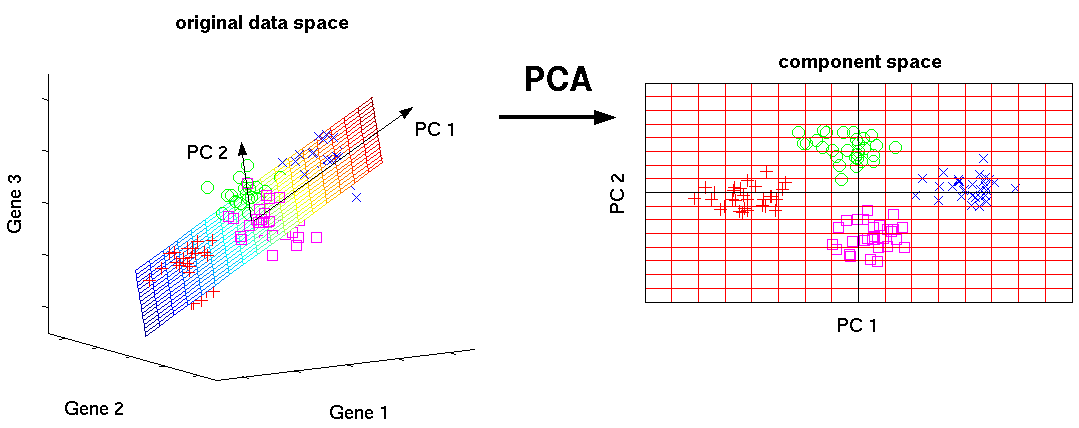
• PCA provides a normalisation that accounts for correlations between features.
• PCA finds a change of basis for the data.
• The first principal component is the direction in which the variance is highest.

second Principal Component orthogonal to the first one

• Everything you did and didn't know about PCA
• article: step-by-step-explanation-of-principal-component-analysis
• video: Principal Component Analysis (PCA)

Eigenfaces

5 Probability 1: Entropy, (Naive) Bayes, Cross-entropy loss (MLVU2019)

Entropy

• A Short Introduction to Entropy, Cross-Entropy and KL-Divergence

6 Linear Models 2: Neural Networks, Backpropagation, SVMs and Kernel methods

backpropagation

• another name for gradiant discent
• Backpropagation is about understanding how changing the weights and biases in a network changes the cost function.
• The goal of backpropagation is to compute the partial derivatives ∂C/∂w and ∂C/∂b of the cost function C with respect to any weight w or bias b in the network.
• Backpropagation is based around four fundamental equations. Together, those equations give us a way of computing both the error δl and the gradient of the cost function.

• source

SVM Soft-margin vs Hard margin

• hard margin works only with fully linear peparable data
• soft margin extends hard margin allowing erorrs to be made fitting the model

Kernel svm

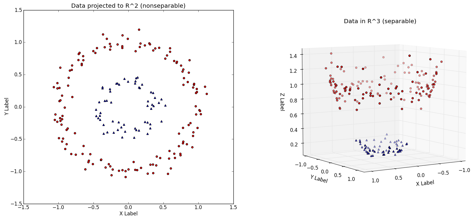
• introduce another axe-z and find a function that allow us to extract common z-axe value for each group of points.
  • Pros: Provides a principled way of solving the multiclass problem.
  • Cons: Multiclass extensions tend to be much more complicated than the original binary

---

9 Deep Learning 2: GANs and VAEs (MLVU2019)

generative adversarial networks

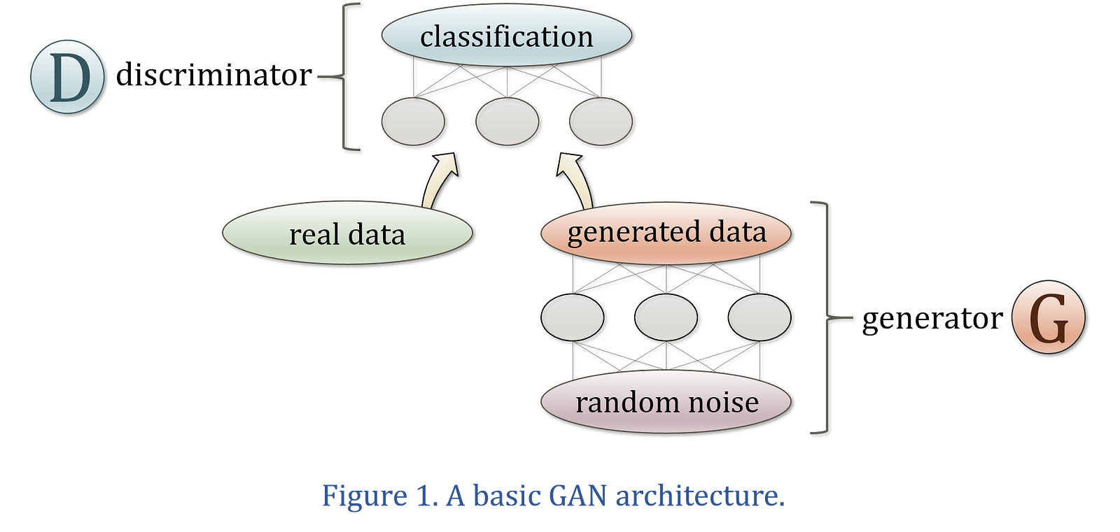
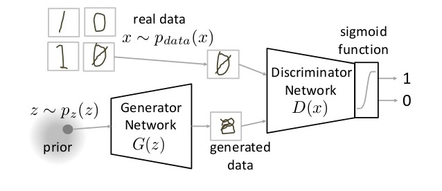
The original GAN was created by Ian Goodfellow, who described the GAN architecture in a paper published in mid-2014. The discriminator tries to determine whether information is real or fake. The other neural network, called a generator, tries to create data that the discriminator thinks is real. We have a generator network and discriminator network playing against each other. The generator tries to produce samples from the desired distribution and the discriminator tries to predict if the sample is from the actual distribution or produced by the generator. The generator and discriminator are trained jointly. The effect this has is that eventually the generator learns to approximate the underlying distribution completely and the discriminator is left guessing randomly.

Vanilla GAN

The original GAN is called a vanilla GAN.

Conditional GAN

CycleGANs

Style GAN

Autoencoders

Autoencoders encode input data as vectors. They create a hidden, or compressed, representation of the raw data. They are useful in dimensionality reduction; that is, the vector serving as a hidden representation compresses the raw data into a smaller number of salient dimensions. Autoencoders can be paired with a so-called decoder, which allows you to reconstruct input data based on its hidden representation, much as you would with a restricted Boltzmann machine.

• useful for image trasmission low-bandwith

Other videos:

• video: Generative Adversarial Networks (GANs) - How and Why They Work
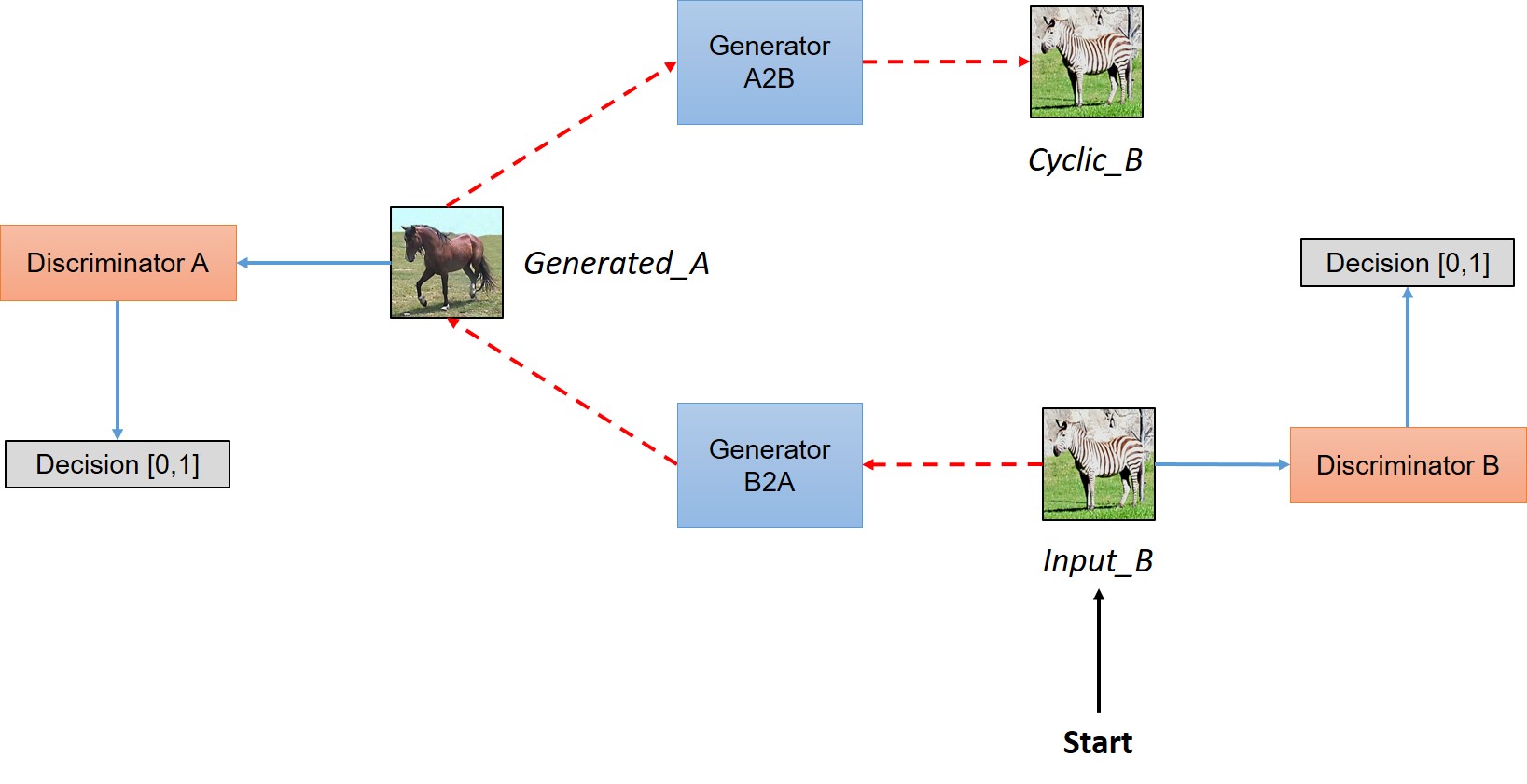
• video: Turning Fortnite into PUBG with Deep Learning (CycleGANs)

---

Which statement is acceptable from a Bayesian perspective, but not from a frequentist perspective?

The frequentists interpretation needs some explanation. Frequentists can assign probabilities only to events/obervations that come from repeatable experiments. With "probability of an event" they mean the relative frequency of the event occuring in an infinitively long series of repetitions. For instance, when a frequentists says that the probability for "heads" in a coin toss is 0.5 (50%) he means that in infinititively many such coin tosses, 50% of the coins will show "head". The difference may become clear when bot (Bayesian frequentist) are asked for the probability that this particular coin I just tossed shows "head". The Bayesian will say: "Since I have no further information than that there are two possible outcomes, I have no reason to prefer any of the sides, so I will assign an equal probability to both of them (what will be 0.5 for "heads" and also 0.5 for "tails").

• Frequentist vs. Bayesian Inference COURSERA

Onehot encoding

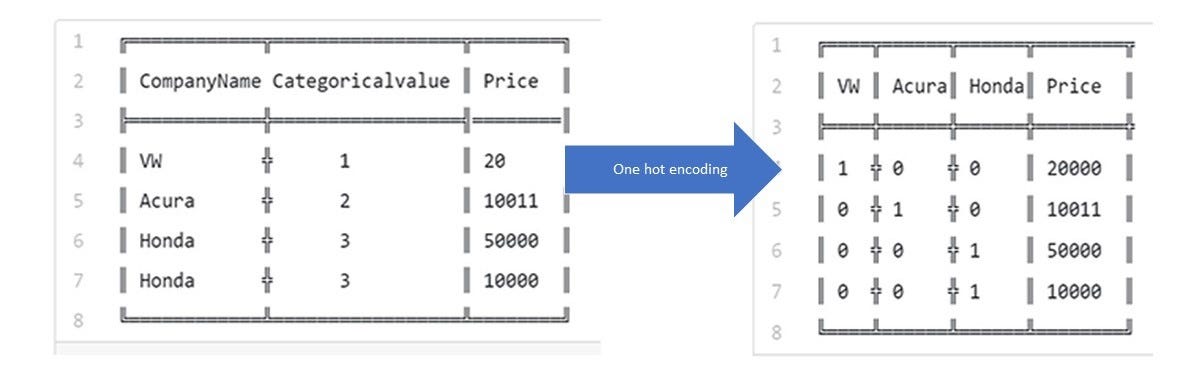
We use one hot encoder to perform “binarization” of the category and include it as a feature to train the model.

Generative VS Discriminative Models

• article: “is this animal a lion or an elephant?”