Visium_SPG_AD

Overview

Welcome to the Visium_SPG_AD project! This project involves several interactive websites, which are publicly accessible for you to browse and download.

We spatially resolved transcriptomics of the inferior temporal cortex (ITC) from postmortem human brain tissue to study local gene expression profiles of brain microenvironments associated with Alzheimer’s disease (AD) related neuropathology bearing abnormal protein aggregation of amyloid beta (Abeta; Ab) and phosphorylated Tau (pTau). Using a total of 10 tissue samples from 3 donors with late-stage Alzheimer’s disease (AD) and 1 age-matched control (Br3874), we generated proteomic-based, spatially-resolved transcriptome-scale (SRT) maps of the human ITC in which the immunofluorescence staining of Ab and pTau was integrated into the complementary SRT data of the identical tissue sections. With Visium Spatial Proteogenomics (Visium-SPG), we utilized a within-subjects design to study gene expression changes associated with spatially localized brain neuropathology across the 3 donors with AD (Br3854, Br3873, and Br3880). Here, using BayesSpace to identify the gray-matter associated spots in a data-driven manner, we discovered statistically significant differentially expressed genes in the core (Ab spots) and peripheral (next_Ab spots) compartments of Ab-associated microenvironment in the gray matter of ITC. For more detailed information about study design and experimental results, please refer to our manuscript. This work was performed by the Keri Martinowich, Kristen Maynard, and Leonardo Collado-Torres teams at the Lieber Institute for Brain Development as well as Stephanie Hicks’s group from JHBSPH’s Biostatistics Department. This project was done in collaboration with 10x Genomics.

This project involves the LieberInstitute/Visium_SPG_AD GitHub repository.

If you tweet about this website, the data or the R package please use the #Visium_SPG_AD hashtag. You can find previous tweets that way as shown here.

Thank you for your interest in our work!

Study Design

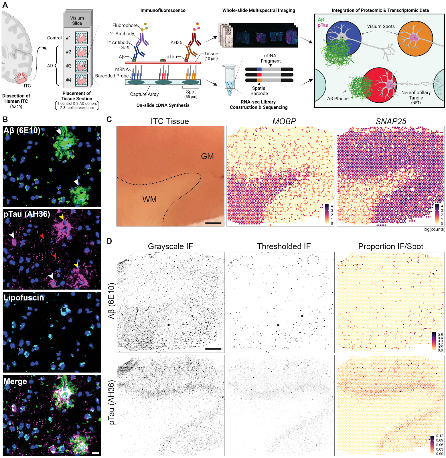
Spatial transcriptomics combined with immunodetection of Ab and pTau in the human inferior temporal cortex (ITC). (A) Schematic of experimental design using Visium Spatial Proteogenomics (Visium-SPG) to investigate the impact of Ab and pTau aggregates on the local microenvironment transcriptome in the post-mortem human brain. Human ITC blocks were acquired from 3 donors with AD and 1 age-matched neurotypical control. Tissue blocks were cryosectioned at 10μm to obtain 2-3 replicates per donor and sections were collected onto individual capture arrays of a Visium spatial gene expression slide, yielding a total of 3 gene expression experiments. The entire slide (4 tissue sections) was stained and scanned using multispectral imaging methods to detect Ab and pTau immunofluorescence (IF) signals as well as autofluorescence. Following imaging, tissue sections were permeabilized and subjected to on-slide cDNA synthesis after which libraries were generated and sequenced. Transcriptomic data was aligned with the respective IF image data to generate gene expression maps of the local transcriptome with respect to Ab plaques and pTau elements, including neurofibrillary tangles. (B) High magnification images show Ab plaques (white triangles) and various neurofibrillary elements such as tangles (white arrowheads), neuropil threads (red arrowheads), and neuritic tau plaques (yellow arrowheads). Lipofuscin (cyan) was identified through spectral unmixing and pixels confounded with this autofluorescent signal were excluded from analysis, scale bar, 20μm. (C) ITC tissue block from Br3880 (left) and corresponding spotplots (right) from the Visium data show gene expression of MOBP and SNAP25, which demarcates the border between gray matter (GM) and white matter (WM), scale bar, 1mm. Color scale indicates spot-level gene expression in logcounts. (D) Image processing and quantification of Ab and pTau per Visium spot. Ab and pTau signals were thresholded in their single IF channels for segmentation against autofluorescence background, including lipofuscin. Thresholded Ab and pTau signals were aligned to the gene expression map of the same tissue section from Br3880 and quantified as the proportion of number of pixels per Visium spot, which is visualized in a spotplot, scale bar, 1mm.

Interactive Websites

All of these interactive websites are powered by open source software, namely:

• 🔭 spatialLIBD
• 👀 iSEE
• 🔍 samui

We provide the following interactive websites, organized by software labeled with emojis:

• 🔭 spatialLIBD
  • Visium_SPG_AD_wholegenome: spatialLIBD website showing the spatially-resolved Visium-SPG data (n = 10 tissue sections from 3 AD donors and 1 age-matched control) with statistical results comparing the 7 different spot categories bearing Ab and pTau pathology within donors with AD. This version shows the whole genome gene expression data.
  • Visium_SPG_AD_TGE: spatialLIBD website that the same as the previous one, but with the targeted gene expression (TGE) panel data.
  • Visium_SPG_AD_wholegenome_Abeta_microenv: spatialLIBD website similar to Visium_SPG_AD_wholegenome, but with the Ab and next_Ab pathologies collapsed into a single one Ab_env for studying the Abeta micro environment.
  • Visium_SPG_AD_wholegenome_Abeta_and_pTau_microenv: spatialLIBD website similar to Visium_SPG_AD_wholegenome_Abeta_microenv, but after also combining pTau and next_pTau into pTau_env as well as both and next_both into both_env, thus resulting in only 4 categories: none, Ab_env, pTau_env, and both_env.
• 👀 iSEE
  • Visium_SPG_AD_pseudobulk_AD_pathology_wholegenome: iSEE website showing the pseudo-bulked spatial data of the 7 different pathological categories.
• 🔍 samui
  • Visium SPG AD on Samui: samui website that allows to zoom in the raw immunostaining image data at the Visium spot level.

Local spatialLIBD apps

If you are interested in running the spatialLIBD applications locally, you can do so thanks to the spatialLIBD::run_app(), which you can also use with your own data as shown in our vignette for publicly available datasets provided by 10x Genomics.

## Run this web application locally with:
spatialLIBD::run_app()
## You will have more control about the length of the session and memory usage.
## See http://research.libd.org/spatialLIBD/reference/run_app.html#examples.
## See also:
## * https://github.com/LieberInstitute/Visium_SPG_AD/tree/master/code/05_deploy_app_wholegenome
## * https://github.com/LieberInstitute/Visium_SPG_AD/tree/master/code/06_deploy_app_targeted
## * https://github.com/LieberInstitute/Visium_SPG_AD/tree/master/code/18_deploy_app_wholegenome_Abeta_microenv
## 
## You could also use spatialLIBD::run_app() to visualize your
## own data given some requirements described
## in detail in the package vignette documentation
## at http://research.libd.org/spatialLIBD/.

Contact

We value public questions, as they allow other users to learn from the answers. If you have any questions, please ask them at LieberInstitute/Visium_SPG_AD/issues and refrain from emailing us. Thank you again for your interest in our work!

Citing our work

Please cite this manuscript if you use data from this project.

Influence of Alzheimer’s disease related neuropathology on local microenvironment gene expression in the human inferior temporal cortex. Sang Ho Kwon, Sowmya Parthiban, Madhavi Tippani, Heena R Divecha, Nicholas J Eagles, Jashandeep S Lobana, Stephen R Williams, Michelle Mark, Rahul A Bharadwaj, Joel E Kleinman, Thomas M Hyde, Stephanie C Page, Stephanie C Hicks, Keri Martinowich, Kristen R Maynard, Leonardo Collado-Torres. GEN Biotechnology; doi: https://doi.org/10.1089/genbio.2023.0019

Below is the citation in BibTeX format.

@article{kwon_influence_2023,
    title = {Influence of {Alzheimer}'s {Disease} {Related} {Neuropathology} on {Local} {Microenvironment} {Gene} {Expression} in the {Human} {Inferior} {Temporal} {Cortex}},
    volume = {2},
    issn = {2768-1572},
    url = {https://liebertpub.com/doi/10.1089/genbio.2023.0019},
    doi = {10.1089/genbio.2023.0019},
    number = {5},
    urldate = {2024-04-19},
    journal = {GEN Biotechnology},
    author = {Kwon, Sang Ho and Parthiban, Sowmya and Tippani, Madhavi and Divecha, Heena R. and Eagles, Nicholas J. and Lobana, Jashandeep S. and Williams, Stephen R. and Mak, Michelle and Bharadwaj, Rahul A. and Kleinman, Joel E. and Hyde, Thomas M. and Page, Stephanie C. and Hicks, Stephanie C. and Martinowich, Keri and Maynard, Kristen R. and Collado-Torres, Leonardo},
    month = oct,
    year = {2023},
    note = {Publisher: Mary Ann Liebert, Inc., publishers},
    pages = {399--417}
}

Cite spatialLIBD

Below is the citation output from using citation('spatialLIBD') in R. Please run this yourself to check for any updates on how to cite spatialLIBD.

print(citation("spatialLIBD")[1], bibtex = TRUE)
#> Pardo B, Spangler A, Weber LM, Hicks SC, Jaffe AE, Martinowich K,
#> Maynard KR, Collado-Torres L (2022). "spatialLIBD: an R/Bioconductor
#> package to visualize spatially-resolved transcriptomics data." _BMC
#> Genomics_. doi:10.1186/s12864-022-08601-w
#> <https://doi.org/10.1186/s12864-022-08601-w>,
#> <https://doi.org/10.1186/s12864-022-08601-w>.
#> 
#> A BibTeX entry for LaTeX users is
#> 
#>   @Article{,
#>     title = {spatialLIBD: an R/Bioconductor package to visualize spatially-resolved transcriptomics data},
#>     author = {Brenda Pardo and Abby Spangler and Lukas M. Weber and Stephanie C. Hicks and Andrew E. Jaffe and Keri Martinowich and Kristen R. Maynard and Leonardo Collado-Torres},
#>     year = {2022},
#>     journal = {BMC Genomics},
#>     doi = {10.1186/s12864-022-08601-w},
#>     url = {https://doi.org/10.1186/s12864-022-08601-w},
#>   }

Please note that the spatialLIBD was only made possible thanks to many other R and bioinformatics software authors, which are cited either in the vignettes and/or the paper(s) describing the package.

Cite VistoSeg

To cite VistoSeg please use:

VistoSeg: {Processing utilities for high-resolution images for spatially resolved transcriptomics data. Madhavi Tippani, Heena R. Divecha, Joseph L. Catallini II, Sang Ho Kwon, Lukas M. Weber, Abby Spangler, Andrew E. Jaffe, Thomas M. Hyde, Joel E. Kleinman, Stephanie C. Hicks, Keri Martinowich, Leonardo Collado-Torres, Stephanie C. Page, Kristen R. Maynard Biological Imaging ; doi: https://doi.org/10.1017/S2633903X23000235

Below is the citation in BibTeX format.

@article{tippani_vistoseg_2023,
    title = {{VistoSeg}: {Processing} utilities for high-resolution images for spatially resolved transcriptomics data},
    volume = {3},
    issn = {2633-903X},
    shorttitle = {{VistoSeg}},
    url = {https://www.cambridge.org/core/journals/biological-imaging/article/vistoseg-processing-utilities-for-highresolution-images-for-spatially-resolved-transcriptomics-data/990CBC4AC069F5EDC62316919398404B},
    doi = {10.1017/S2633903X23000235},
    language = {en},
    urldate = {2024-04-19},
    journal = {Biological Imaging},
    author = {Tippani, Madhavi and Divecha, Heena R. and Catallini, Joseph L. and Kwon, Sang H. and Weber, Lukas M. and Spangler, Abby and Jaffe, Andrew E. and Hyde, Thomas M. and Kleinman, Joel E. and Hicks, Stephanie C. and Martinowich, Keri and Collado-Torres, Leonardo and Page, Stephanie C. and Maynard, Kristen R.},
    month = jan,
    year = {2023},
    keywords = {hematoxylin and eosin, immunofluorescence, MATLAB, segmentation, spatially resolved transcriptomics, Visium, Visium-Spatial Proteogenomics},
    pages = {e23}
}

Data Access

We highly value open data sharing and believe that doing so accelerates science, as was the case between our HumanPilot and the external BayesSpace projects, documented on this slide.

Processed Data

spatialLIBD also allows you to access the data from this project as ready to use R objects. That is, a:

• SpatialExperiment object for the Visium-SPG samples (n = 10)

You can use the zellkonverter Bioconductor package to convert any of them into Python AnnData objects. If you browse our code, you can find examples of such conversions.

If you are unfamiliar with these tools, you might want to check the LIBD rstats club (check and search keywords on the schedule) videos and resources.

Installing spatialLIBD

Get the latest stable R release from CRAN. Then install spatialLIBD from Bioconductor with the following code:

## Install BiocManager in order to install Bioconductor packages properly
if (!requireNamespace("BiocManager", quietly = TRUE)) {
    install.packages("BiocManager")
}
## Check that you have a valid R/Bioconductor installation
BiocManager::valid()
## Now install spatialLIBD from Bioconductor
## (this version has been tested on macOS, winOS, linux)
BiocManager::install("spatialLIBD")
## If you need the development version from GitHub you can use the following:
# BiocManager::install("LieberInstitute/spatialLIBD")
## Note that this version might include changes that have not been tested
## properly on all operating systems.

R objects

Using spatialLIBD you can access the spatialDLPFC transcriptomics data from the 10x Genomics Visium platform. For example, this is the code you can use to access the spatially-resolved data. For more details, check the help file for fetch_data().

As of August 23, 2023 the processed data includes spot-level deconvolution results generated using cell2location with the six broad cell types from the Mathys et al snRNA-seq dataset in which they found AD associated gene expression changes. To access these results check the colData(spe) columns starting with the c2l_ prefix.

## Check that you have a recent version of spatialLIBD installed
stopifnot(packageVersion("spatialLIBD") >= "1.11.12")
## Download the spot-level data
spe <- spatialLIBD::fetch_data(type = "Visium_SPG_AD_Visium_wholegenome_spe")

## This is a SpatialExperiment object
spe
#> class: SpatialExperiment 
#> dim: 27853 38115 
#> metadata(0):
#> assays(2): counts logcounts
#> rownames(27853): ENSG00000243485 ENSG00000238009 ... ENSG00000278817
#>   ENSG00000277196
#> rowData names(7): source type ... gene_type gene_search
#> colnames(38115): AAACAACGAATAGTTC-1 AAACAAGTATCTCCCA-1 ...
#>   TTGTTTGTATTACACG-1 TTGTTTGTGTAAATTC-1
#> colData names(113): key sample_id ... c2l_oli c2l_opc
#> reducedDimNames(15): 10x_pca 10x_tsne ... TSNE_perplexity50.HARMONY
#>   TSNE_perplexity80.HARMONY
#> mainExpName: NULL
#> altExpNames(0):
#> spatialCoords names(2) : pxl_col_in_fullres pxl_row_in_fullres
#> imgData names(4): sample_id image_id data scaleFactor
lobstr::obj_size(spe)
#> 2.29 GB

## Remake the logo image
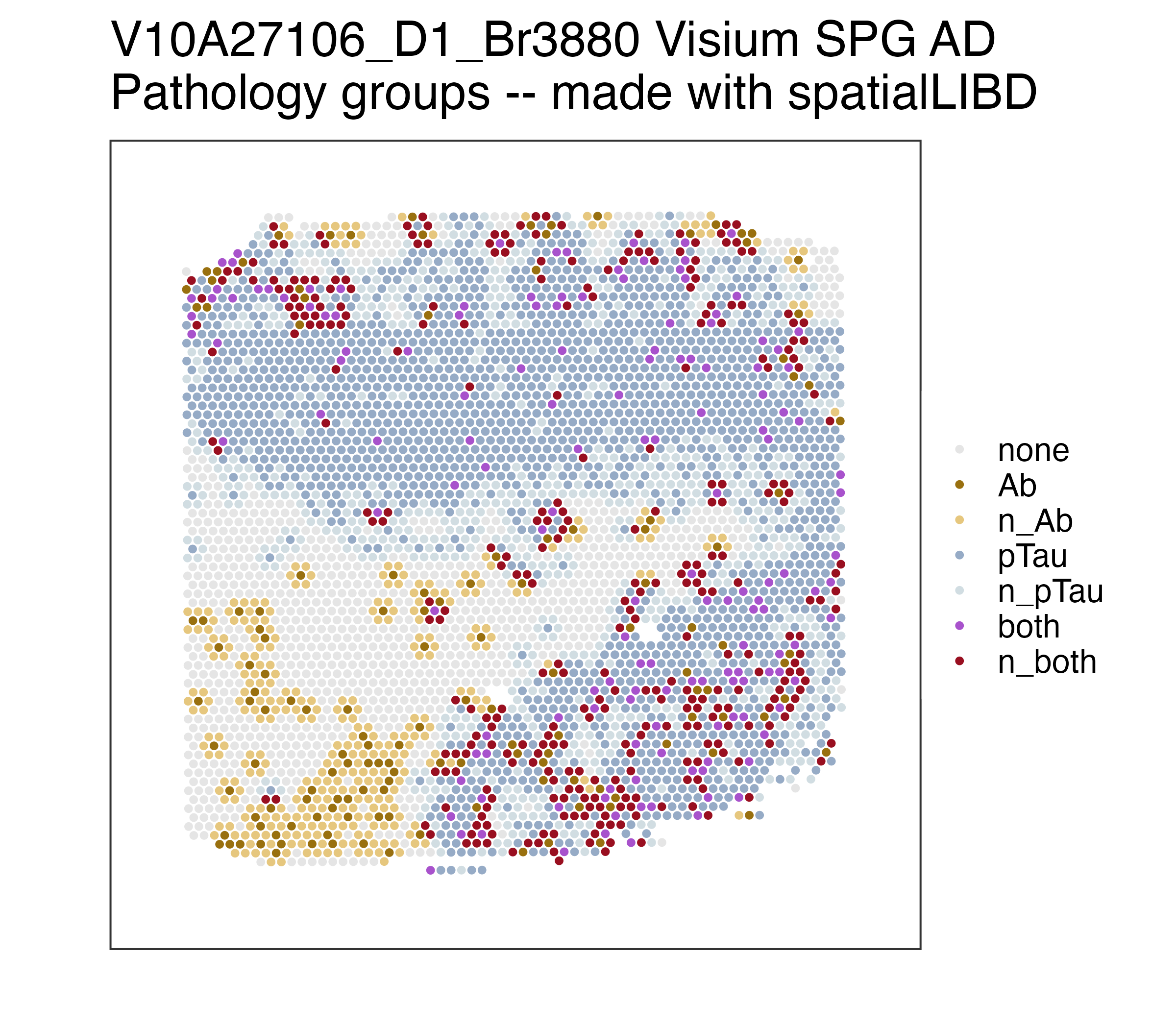
p_pathology <- spatialLIBD::vis_clus(
    spe = spe,
    clustervar = "path_groups",
    sampleid = "V10A27106_D1_Br3880",
    colors = spe$path_groups_colors[!duplicated(spe$path_groups_colors)],
    spatial = FALSE,
    ... = " Visium SPG AD\nPathology groups -- made with spatialLIBD"
)
p_pathology

## Repeat but for BayesSpace at k = 28 (max 28 clusters, can be less)
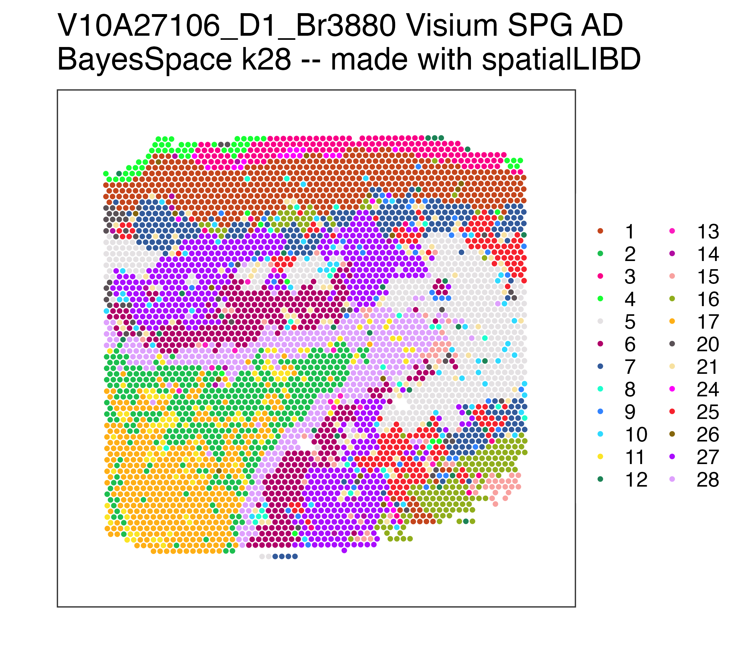
k_observed <- unique(spe$BayesSpace_harmony_k28)
p_BayesSpace <- spatialLIBD::vis_clus(
    spe = spe,
    clustervar = "BayesSpace_harmony_k28",
    sampleid = "V10A27106_D1_Br3880",
    spatial = FALSE,
    colors = setNames(Polychrome::palette36.colors(length(k_observed)), k_observed),
    ... = " Visium SPG AD\nBayesSpace k28 -- made with spatialLIBD"
)
p_BayesSpace

Raw data

You can access all the raw data through Globus (jhpce#Visium_SPG_AD). This includes all the input FASTQ files as well as the outputs from tools such as SpaceRanger. The files are organized following the LieberInstitute/template_project project structure.

Internal

• JHPCE locations: /dcs04/lieber/lcolladotor/with10x_LIBD001/Visium_SPG_AD
• Slack channel: libd_visium_if_ad_itg.

Files:

• code: R, python, and shell scripts for running various analyses.
• plots: plots generated by R analysis scripts in .pdf or .png format
• processed-data
  • Images: images used for running SpaceRanger and other images
  • spaceranger: SpaceRanger output files
• raw-data
  • 10x_files: files 10x Genomics transferred to us.
  • FASTQ: FASTQ files.
  • Images: raw images from the scanner in .tif format for each Visium-SPG slide (around 8GB each). Each slide contains the image for four capture areas.

This GitHub repository is organized along the R/Bioconductor-powered Team Data Science group guidelines. It follows the LieberInstitute/template_project structure.

Other related files

• Reference transcriptome from 10x Genomics: /dcs04/lieber/lcolladotor/annotationFiles_LIBD001/10x/refdata-gex-GRCh38-2020-A/