Links: Github Page | Documentation | Github | PyPi - project | _ Installation: pip install pylfsr
- New Updates
- Installation
- Examples
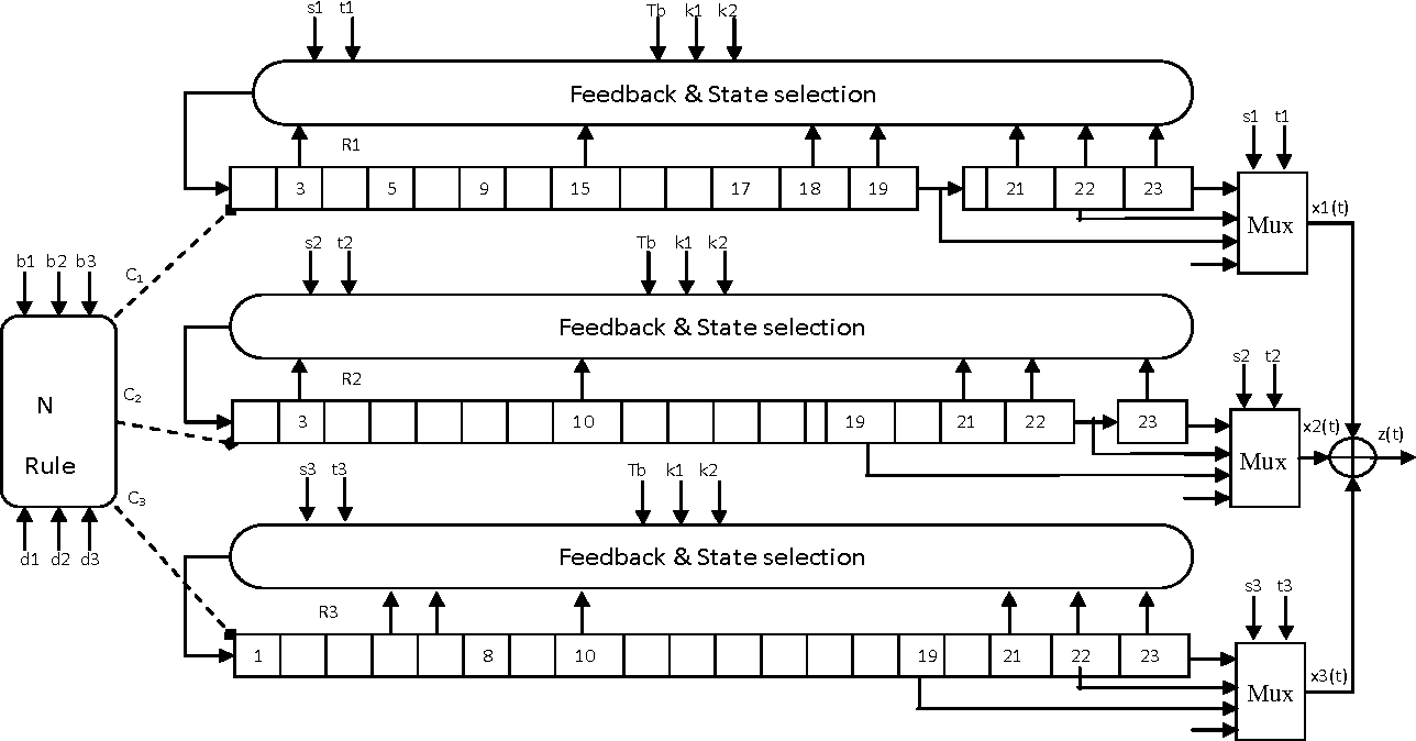
- A5/1 GSM Stream Cipher
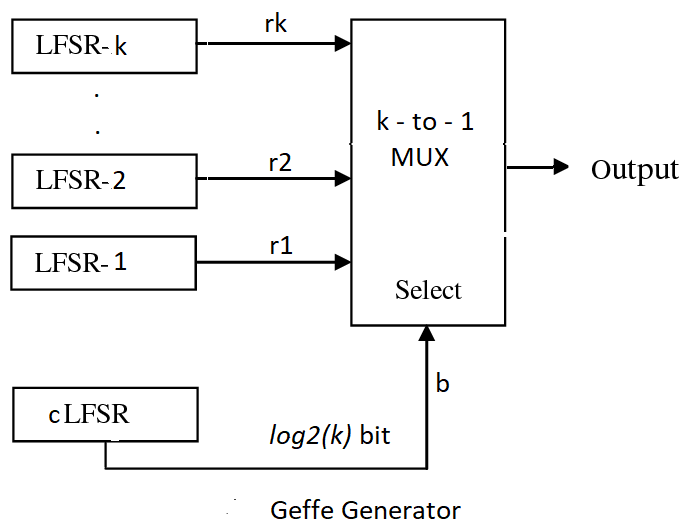
- Geffe Genegerator
- Matlab Implementation
- Cite As
Version: 1.0.7:
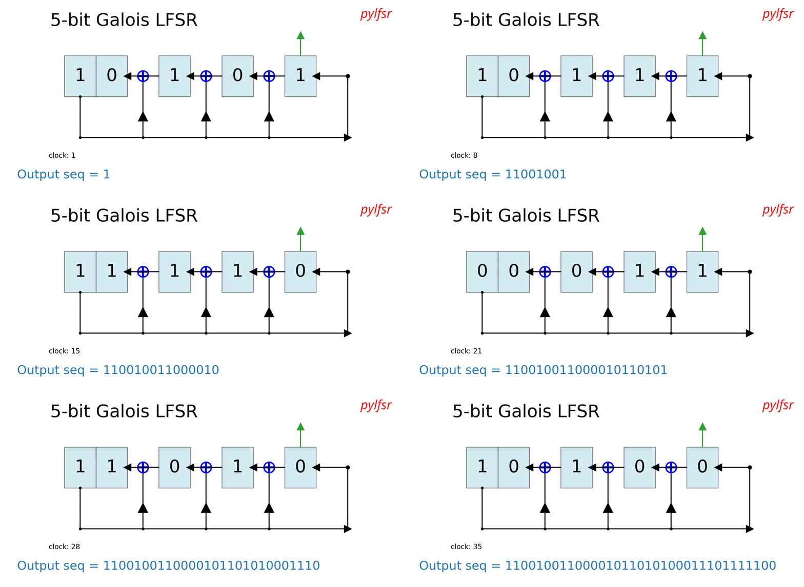
- Added Galois Configuration
- Improved Documentation
- Computing LZ complexity
Version: 1.0.6:
- Fixed the bugs (1) missing initial bit (2) exception
- Added test properties of LFSR
- (1) Balance Property
- (2) Runlength Property
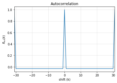
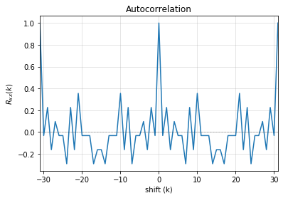
- (3) Autocorrelation Property
- Ploting function to display LFSR
- A5/1 GSM Stream Ciper Generator
- Geffe Generator
pip install pylfsr
conda install -c nikeshbajaj pylfsr
in process of including in conda-forge
Download the repository or clone it with git, after cd in directory build it from source with
python setup.py install
# import LFSR
import numpy as np
from pylfsr import LFSR

L = LFSR()

# print the info
L.info()

5 bit LFSR with feedback polynomial  x^5 + x^2 + 1
Expected Period (if polynomial is primitive) =  31
Current :
State        :  [1 1 1 1 1]
Count        :  0
Output bit   : -1
feedback bit : -1
L.next()
L.runKCycle(10)
L.runFullCycle()
L.info()
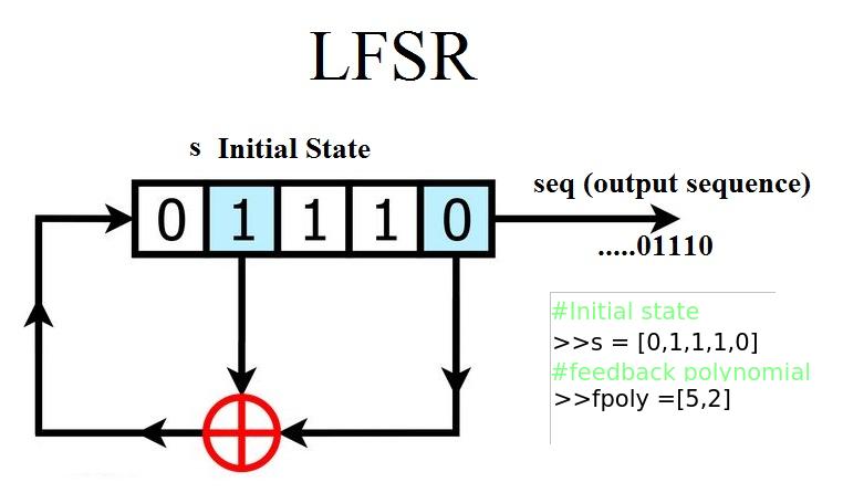
state = [0,0,0,1,0]
fpoly = [5,4,3,2]
L = LFSR(fpoly=fpoly,initstate =state, verbose=True)
L.info()
tempseq = L.runKCycle(10)
L.set(fpoly=[5,3])
state = [1,1,1]
fpoly = [3,2]
L = LFSR(initstate=state,fpoly=fpoly)
print('count \t state \t\toutbit \t seq')
print('-'*50)
for _ in range(15):
    print(L.count,L.state,'',L.outbit,L.seq,sep='\t')
    L.next()
print('-'*50)
print('Output: ',L.seq)
Output :
count 	        state 		outbit 	 seq
--------------------------------------------------
0		[1 1 1]		-1	[-1]
1		[0 1 1]		1	[1]
2		[0 0 1]		1	[1 1]
3		[1 0 0]		1	[1 1 1]
4		[0 1 0]		0	[1 1 1 0]
5		[1 0 1]		0	[1 1 1 0 0]
6		[1 1 0]		1	[1 1 1 0 0 1]
7		[1 1 1]		0	[1 1 1 0 0 1 0]
8		[0 1 1]		1	[1 1 1 0 0 1 0 1]
9		[0 0 1]		1	[1 1 1 0 0 1 0 1 1]
10		[1 0 0]		1	[1 1 1 0 0 1 0 1 1 1]
11		[0 1 0]		0	[1 1 1 0 0 1 0 1 1 1 0]
12		[1 0 1]		0	[1 1 1 0 0 1 0 1 1 1 0 0]
13		[1 1 0]		1	[1 1 1 0 0 1 0 1 1 1 0 0 1]
14		[1 1 1]		0	[1 1 1 0 0 1 0 1 1 1 0 0 1 0]
--------------------------------------------------
Output:  [1 1 1 0 0 1 0 1 1 1 0 0 1 0 1]
state = [1,1,1]
fpoly = [3,2]
L = LFSR(initstate=state,fpoly=fpoly,counter_start_zero=False)
print('count \t state \t\toutbit \t seq')
print('-'*50)
for _ in range(15):
    print(L.count,L.state,'',L.outbit,L.seq,sep='\t')
    L.next()
print('-'*50)
print('Output: ',L.seq)
Output
count 	 state 		outbit 	 seq
--------------------------------------------------
1	[1 1 1]		1	[1]
2	[0 1 1]		1	[1 1]
3	[0 0 1]		1	[1 1 1]
4	[1 0 0]		0	[1 1 1 0]
5	[0 1 0]		0	[1 1 1 0 0]
6	[1 0 1]		1	[1 1 1 0 0 1]
7	[1 1 0]		0	[1 1 1 0 0 1 0]
8	[1 1 1]		1	[1 1 1 0 0 1 0 1]
9	[0 1 1]		1	[1 1 1 0 0 1 0 1 1]
10	[0 0 1]		1	[1 1 1 0 0 1 0 1 1 1]
11	[1 0 0]		0	[1 1 1 0 0 1 0 1 1 1 0]
12	[0 1 0]		0	[1 1 1 0 0 1 0 1 1 1 0 0]
13	[1 0 1]		1	[1 1 1 0 0 1 0 1 1 1 0 0 1]
14	[1 1 0]		0	[1 1 1 0 0 1 0 1 1 1 0 0 1 0]
--------------------------------------------------
Output:  [1 1 1 0 0 1 0 1 1 1 0 0 1 0 1]
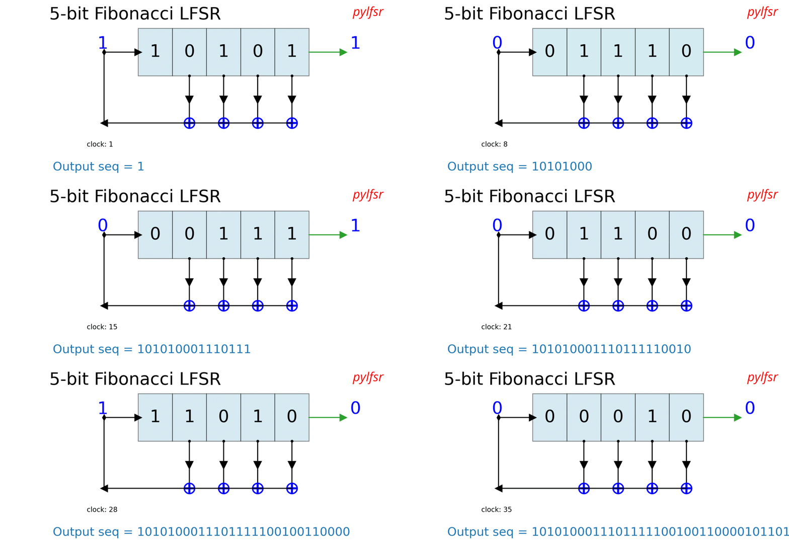
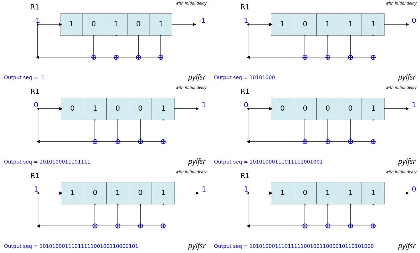
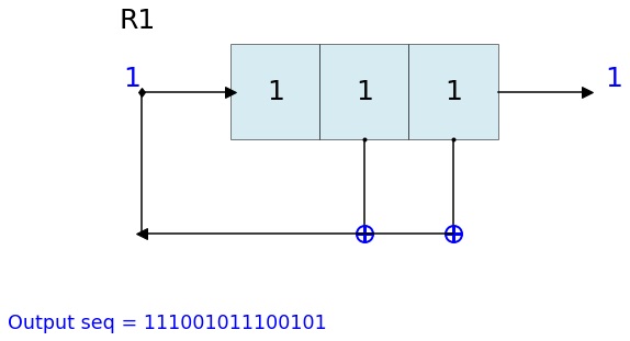
L.Viz(show=False, show_labels=False,title='R1')
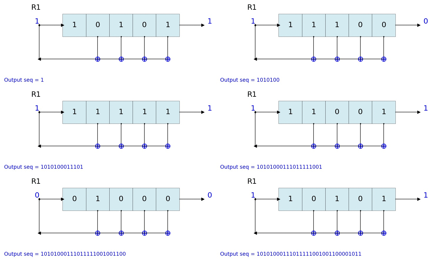
%matplotlib notebook
L = LFSR(initstate=[1,0,1,0,1],fpoly=[5,4,3,2],counter_start_zero=False)
fig, ax = plt.subplots(figsize=(8,3))
for _ in range(35):
  ax.clear()
  L.Viz(ax=ax, title='R1')
  plt.ylim([-0.1,None])
  #plt.tight_layout()
  L.next()
  fig.canvas.draw()
  plt.pause(0.1)
fpoly = [23,19]
L1 = LFSR(fpoly=fpoly,initstate ='ones', verbose=False)
L1.info()
Output
23 bit LFSR with feedback polynomial  x^23 + x^19 + 1
Expected Period (if polynomial is primitive) =  8388607
Current :
 State        :  [1 1 1 1 1 1 1 1 1 1 1 1 1 1 1 1 1 1 1 1 1 1 1]
 Count        :  0
 Output bit   :  -1
 feedback bit :  -1
seq = L1.runKCycle(100)
array([1, 1, 1, 1, 1, 1, 1, 1, 1, 1, 1, 1, 1, 1, 1, 1, 1, 1, 1, 1, 1, 1,
1, 0, 0, 0, 0, 0, 0, 0, 0, 0, 0, 0, 0, 0, 0, 0, 0, 0, 0, 0, 1, 1,
1, 1, 0, 0, 0, 0, 0, 0, 0, 0, 0, 0, 0, 0, 0, 0, 0, 1, 1, 1, 1, 1,
1, 1, 1, 0, 0, 0, 0, 0, 0, 0, 0, 0, 0, 0, 1, 1, 1, 1, 0, 0, 0, 0,
1, 1, 1, 1, 0, 0, 0, 0, 0, 0, 0, 1])
state = [1,1,1,1,0]
fpoly = [5,3]
L = LFSR(initstate=state,fpoly=fpoly)
result  = L.test_properties(verbose=2)
Output
1. Periodicity
------------------
 - Expected period = 2^M-1 = 31
 - Pass?:  True

2. Balance Property
-------------------
 - Number of 1s = Number of 0s+1 (in a period): (N1s,N0s) =  (16, 15)
 - Pass?:  True

3. Runlength Property
-------------------
 - Number of Runs in a period should be of specific order, e.g. [4,2,1,1]
 - Runs:  [8 4 2 1 1]
 - Pass?:  True

4. Autocorrelation Property
-------------------
 - Autocorrelation of a period should be noise-like, specifically, 1 at k=0, -1/m everywhere else
 - Pass?:  True

==================
Passed all the tests
==================
Testing individual property
# get a full period sequence
p = L.getFullPeriod()
p
array([0, 1, 1, 1, 1, 1, 0, 0, 0, 1, 1, 0, 1, 1, 1, 0, 1, 0, 1, 0, 0, 0,
       0, 1, 0, 0, 1, 0, 1, 1, 0])
L.balance_property(p.copy())
# (True, (16, 15))

L.runlength_property(p.copy())
# (True, array([8, 4, 2, 1, 1]))

L.autocorr_property(p.copy())[0]
#True
state = [1,1,1,1,0]
fpoly = [5,1]
L = LFSR(initstate=state,fpoly=fpoly)
result = L.test_properties(verbose=1)
Output
1. Periodicity
------------------
 - Expected period = 2^M-1 = 31
 - Pass?:  False

2. Balance Property
-------------------
 - Number of 1s = Number of 0s+1 (in a period): (N1s,N0s) =  (17, 14)
 - Pass?:  False

3. Runlength Property
-------------------
 - Number of Runs in a period should be of specific order, e.g. [4,2,1,1]
 - Runs:  [10  2  1  1  2]
 - Pass?:  False

4. Autocorrelation Property
-------------------
 - Autocorrelation of a period should be noise-like, specifically, 1 at k=0, -1/m everywhere else
 - Pass?:  False

==================
Failed one or more tests, check if feedback polynomial is primitive polynomial
==================
Reference : http://www.partow.net/programming/polynomials/index.html
L = LFSR()
# list of 5-bit feedback polynomials
fpoly = L.get_fpolyList(m=5)

# list of all feedback polynomials as a dictionary
fpolyDict = L.get_fpolyList()
L.changeFpoly(newfpoly =[23,14],reset=False)
seq1 = L.runKCycle(20)

# Change after 20 clocks
L.changeFpoly(newfpoly =[23,9],reset=False)
seq2 = L.runKCycle(20)
Ref: https://en.wikipedia.org/wiki/A5/1
import numpy as np
import matplotlib.pyplot as plt
from pylfsr import A5_1

A5 = A5_1(key='random')
print('key: ',A5.key)
A5.R1.Viz(title='R1')
A5.R2.Viz(title='R2')
A5.R3.Viz(title='R3')

print('key: ',A5.key)
print()
print('count \t cbit\t\tclk\t R1_R2_R3\toutbit \t seq')
print('-'*80)
for _ in range(15):
    print(A5.count,A5.getCbits(),A5.clock_bit,A5.getLastbits(),A5.outbit,A5.getSeq(),sep='\t')
    A5.next()
print('-'*80)
print('Output: ',A5.seq)

A5.runKCycle(1000)
A5.getSeq()
Reference Article: Enhancement of A5/1: https://doi.org/10.1109/ETNCC.2011.5958486
# Three LFSRs initialzed with 'ones' though they are intialized with encription key
R1 = LFSR(fpoly = [19,18,17,14])
R2 = LFSR(fpoly = [23,22,21,8])
R3 = LFSR(fpoly = [22,21])

# clocking bits
b1 = R1.state[8]
b2 = R3.state[10]
b3 = R3.state[10]
Ref: Schneier, Bruce. Applied cryptography: protocols, algorithms, and source code in C. john wiley & sons, 2007. Chaper 16
import numpy as np
import matplotlib.pyplot as plt
from pylfsr import Geffe, LFSR

kLFSR = [LFSR(initstate='random') for _ in range(8)]  # List of 8 5-bit LFSRs with default feedback polynomial and random initial state
cLFSR = LFSR(initstate='random')                      # A 5-bit LFSR with for selecting one of 8 output at a time

GG = Geffe(kLFSR_list=kLFSR, cLFSR=cLFSR)

print('key: ',GG.getState())
print()
for _ in range(50):
    print(GG.count,GG.m_count,GG.outbit_k,GG.sel_k,GG.outbit,GG.getSeq(),sep='\t')
    GG.next()

GG.runKCycle(1000)
GG.getSeq()
Folder : https://github.com/Nikeshbajaj/Linear_Feedback_Shift_Register/tree/master/matlabfiles
Description Genrate randon binary sequence using LFSR for any given feedback taps (polynomial), This will also check Three fundamental Property of LFSR
- Balance Property
- Runlength Property
- Autocorrelation Property
This MATLAB Code work for any length of LFSR with given taps (feedback polynomial) -Universal, There are three files LFSRv1.m an LFSRv2.m, LFSRv3.m
This function will return all the states of LFSR and will check Three fundamental Property of LFSR (1) Balance Property (2) Runlength Property (3) Autocorrelation Property
s=[1 1 0 0 1]
t=[5 2]
[seq c] =LFSRv1(s,t)
This function will return only generated sequence will all the states of LFSR, no verification of properties are done here. Use this function to avoid verification each time you execute the program.
s=[1 1 0 0 1]
t=[5 2]
[seq c] =LFSRv2(s,t)
seq = LFSRv3(s,t,N) this function generates N bit sequence only. This is faster then other two functions, as this does not gives each state of LFSR
s=[1 1 0 0 1]
t=[5 2]
seq =LFSRv3(s,t,50)
- If you want to use this function in middle of any program, use LFSRv2 or LFSRv1 with verification =0.
- If you want to make it fast for long length of LFSR,use LFSRv3.m
@software{nikesh_bajaj_2021_4726667,
  author       = {Nikesh Bajaj},
  title        = {Nikeshbajaj/Linear\_Feedback\_Shift\_Register: 1.0.6},
  month        = apr,
  year         = 2021,
  publisher    = {Zenodo},
  version      = {1.0.6},
  doi          = {10.5281/zenodo.4726667},
  url          = {https://doi.org/10.5281/zenodo.4726667}
}
If any doubt, confusion or feedback please contact me
- Nikesh Bajaj
- http://nikeshbajaj.in
- n.bajaj@imperial.ac.uk
- n.bajaj@qmul.ac.uk
- bajaj[dot]nikkey[AT]gmail[dot]?
You will be redirected to https://pylfsr.github.io!


