
pycvodes provides a
Python binding to the
Ordinary Differential Equation
integration routines from cvodes in the
SUNDIALS suite. pycvodes allows a user to numerically integrate
(systems of) differential equations. Note that routines for sensitivity analysis is not yet exposed in this binding (which makes
the functionality essentially the same as cvode).
The following multistep methods are available:
bdf: Backward differentiation formula (of order 1 to 5)adams: implicit Adams method (order 1 to 12)
Note that bdf (as an implicit stepper) requires a user supplied callback for calculating the jacobian.
You may also want to know that you can use pycvodes from
pyodesys
which can e.g. derive the Jacobian analytically (using SymPy). Pyodesys also provides
plotting functions, C++ code-generation and more.
Autogenerated API documentation for latest stable release is found here: https://bjodah.github.io/pycvodes/latest (and the development version for the current master branch are found here: http://hera.physchem.kth.se/~pycvodes/branches/master/html).
Simplest way to install is to use the conda package manager and install the prebuilt binary from the Conda Forge channel. We recommend installing into a conda environment with only packages from Conda Forge:
$ conda create -n pycvodes -c conda-forge pycvodes pytest
$ conda activate pycvodes
(pycvodes)$ python -m pytest --pyargs pycvodes
tests should pass.
Binary distribution is available here: https://anaconda.org/bjodah/pycvodes
Source distribution is available here: https://pypi.python.org/pypi/pycvodes
When installing from source you can choose what lapack lib to link against by setting
the environment variable PYCVODES_LAPACK, your choice can later be accessed from python:
>>> from pycvodes import config
>>> config['LAPACK']  # doctest: +SKIP
'lapack,blas'
If you use pip to install pycvodes, note that prior to installing pycvodes, you will need
to install sundials (pycvodes>=0.12.0 requires sundials>=5.1.0, pycvodes<0.12 requires sundials<5)
and its development headers, with cvodes & lapack enabled
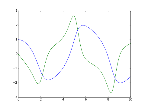
The classic van der Pol oscillator (see examples/van_der_pol.py)
>>> import numpy as np
>>> from pycvodes import integrate_predefined  # also: integrate_adaptive
>>> mu = 1.0
>>> def f(t, y, dydt):
...     dydt[0] = y[1]
...     dydt[1] = -y[0] + mu*y[1]*(1 - y[0]**2)
...
>>> def j(t, y, Jmat, dfdt=None, fy=None):
...     Jmat[0, 0] = 0
...     Jmat[0, 1] = 1
...     Jmat[1, 0] = -1 - mu*2*y[1]*y[0]
...     Jmat[1, 1] = mu*(1 - y[0]**2)
...     if dfdt is not None:
...         dfdt[:] = 0
...
>>> y0 = [1, 0]; dt0=1e-8; t0=0.0; atol=1e-8; rtol=1e-8
>>> tout = np.linspace(0, 10.0, 200)
>>> yout, info = integrate_predefined(f, j, y0, tout, atol, rtol, dt0,
...                                   method='bdf')
>>> import matplotlib.pyplot as plt
>>> series = plt.plot(tout, yout)
>>> plt.show()  # doctest: +SKIP
For more examples see examples/, and rendered jupyter notebooks here: http://hera.physchem.kth.se/~pycvodes/branches/master/examples
The source code is Open Source and is released under the simplified 2-clause BSD license. See LICENSE for further details.
Contributors are welcome to suggest improvements at https://github.com/bjodah/pycvodes
Björn I. Dahlgren, contact:
- gmail address: bjodah
See file AUTHORS in root for a list of all authors.
