-
Notifications
You must be signed in to change notification settings - Fork 32
3D Dai Woodward
This test highlights the ability of a code to resolve all seven MHD waves. Parameters from Dai & Woodward 1998. For more testing information see MHD Riemann Problems. The test consists of two initally moving states (on left pressure is equal to 0.95 and density is equal to 1.08; on right they are both equal 1.0) separated by a discontinuity at 0.5. The left side has a magnetic field of 0.5641895835477563 cholla/builds/make.type.mhd).
#
# Parameter File for 3D Dai & Woodward MHD shock tube
# Citation: Dai & Woodward 1998 "On The Diverrgence-Free Condition and
# Conservation Laws in Numerical Simulations for Supersonic Magnetohydrodynamic
# Flows"
#

################################################
# number of grid cells in the x dimension
nx=256
# number of grid cells in the y dimension
ny=256
# number of grid cells in the z dimension
nz=256
# final output time
tout=0.2
# time interval for output
outstep=0.2
# name of initial conditions
init=Riemann

# domain properties
xmin=0.0
ymin=0.0
zmin=0.0
xlen=1.0
ylen=1.0
zlen=1.0

# type of boundary conditions
xl_bcnd=3
xu_bcnd=3
yl_bcnd=3
yu_bcnd=3
zl_bcnd=3
zu_bcnd=3

# path to output directory
outdir=./

#################################################
# Parameters for 1D Riemann problems
# density of left state
rho_l=1.08
# velocity of left state
vx_l=1.2
vy_l=0.01
vz_l=0.5
# pressure of left state
P_l=0.95
# Magnetic field of the left state
Bx_l=0.5641895835477563
By_l=1.0155412503859613
Bz_l=0.5641895835477563

# density of right state
rho_r=1.0
# velocity of right state
vx_r=0.0
vy_r=0.0
vz_r=0.0
# pressure of right state
P_r=1.0
# Magnetic field of the right state
Bx_r=0.5641895835477563
By_r=1.1283791670955126
Bz_r=0.5641895835477563

# location of initial discontinuity
diaph=0.5
# value of gamma
gamma=1.6666666666666667
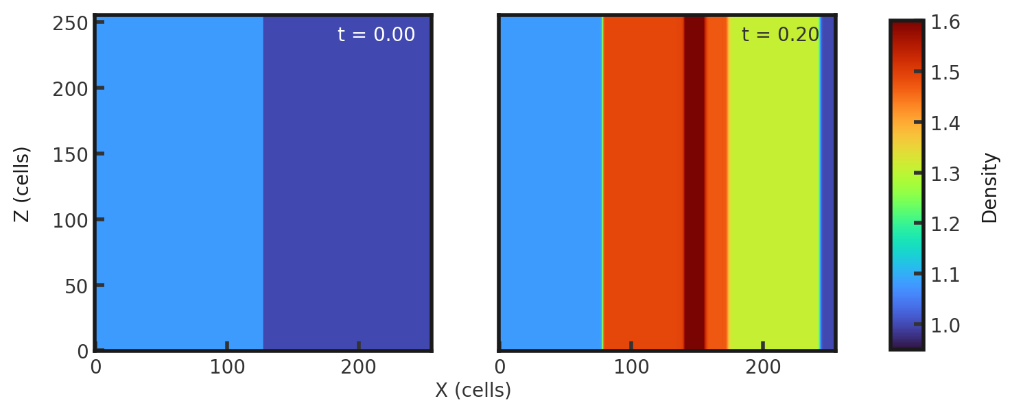
Upon completion, you should obtain two output files. The initial and final densities (in code units) of a slice along the y-midplane is shown below. Examples of how to plot projections and slices can be found in cholla/python_scripts/Projection_Slice_Tutorial.ipynb.
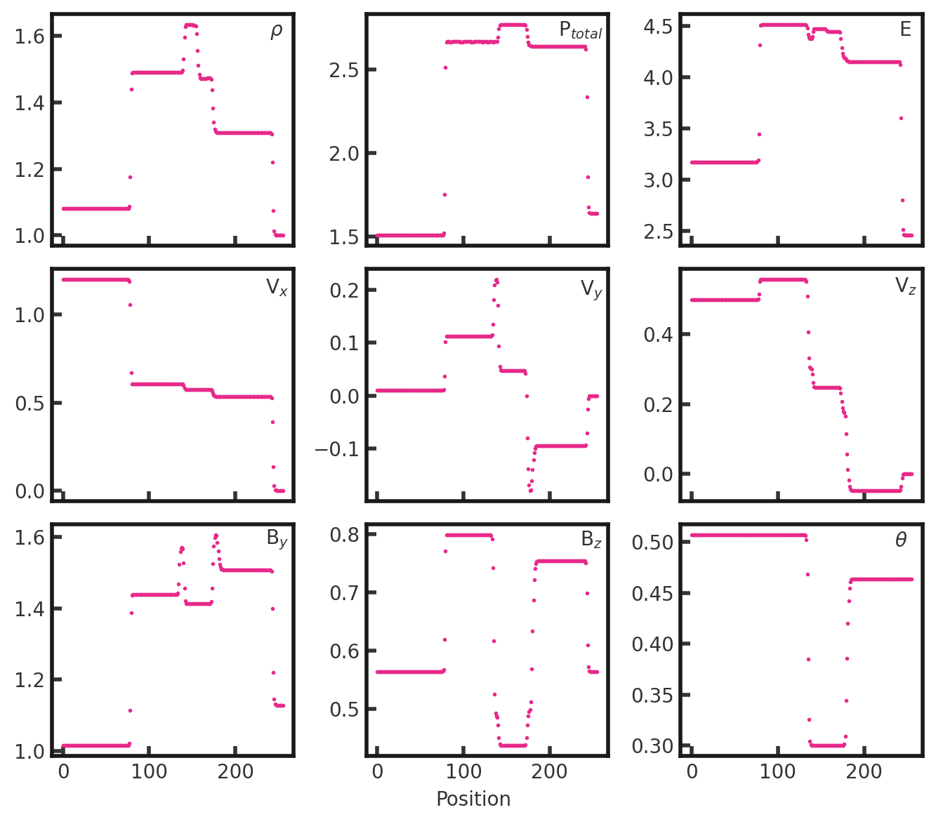
 A skewer in x along y and z midplanes yields the 1-dimensional solution. $\theta$ is defined as $\tan^{-1}\left( \frac{B_{z}}{B_{y}}\right)$:
 We can compare to Miniati & Martin 2011 (note that they are plotting gas pressure, not total pressure):
 From left to right, we see a fast shock followed by Alfven/rotation waves, a slow shock, contact discontinuity, slow shock, alfven/roation waves, and a fast shock