CA-parameter-tuning

Optimizing geometrical cuts during the pixel seeding step of the CMS High-Level Trigger

Prerequisites

Setting up CMSSSW

scram p -n cmssw CMSSW_13_2_0
cd cmssw/src
cmsenv
git cms-merge-topic cms-pixel-autotuning:autotuning
scram b -j 4

Creating a Python environment

Install miniconda, then:

conda create -n [env-name] -c conda-forge -y python=3.9 jupyter numpy pandas matplotlib uproot
conda activate [env-name]

Installing The-Optimizer package

The package can be cloned anywhere, but your conda environment must be active during installation

git clone https://github.com/cms-patatrack/The-Optimizer.git
git checkout pixel-autotuning
pip install .

Setting up this repo

Clone the repo:

git clone https://github.com/cms-pixel-autotuning/CA-parameter-tuning.git
cd CA-parameter-tuning

For Phase-1, there is a script inside the input folder that generates the ttbar events used in our optimization. Simply run

cd input
. generate_input

For other workflows and Phase-2, copy the root file(s) produced in step 2 of the workflow to the input folder.

Running Multi-Objective Particle Swarm Optimization (MOPSO)

You can run the whole thing with python optimize.py and the following options:

• -p2: run the optimization with Phase-2 configuration (Phase-2 input is required)
• -d: calculate efficiency and fake rate corresponding to the default cuts that are currently set in CMSSW
• -e [int]: number of events to process (<=1000)
• -i [int]: number of iterations to run
• -p [int]: number of particles to be spawned
• -c [int]: continue for a number of iterations (a checkpoint folder from a previous run is required)

Results:

The checkpoint folder

This folder contains all the information needed to continue a run. The pareto front, which is what we're looking for, is also included.

• pareto_front.csv: the non-dominated solutions across all iterations. Each row corresponds to a particle on the pareto front. The last two columns are 1 - efficiency and fake rate, while the rest are the cuts (see Phase-1 config or Phase-2 config to know exactly which cut each column corresponds to)
• default.csv: one row containing the default cuts and the corresponding 1 - efficiency and fake rate. The columns are the same as in pareto_front.csv
• individual_states.csv: the current state of the particles. Each row corresponds to one particle, with the columns being its position, velocity, best position, and best fitness
• pso_attributes.json: MOPSO parameters and the number of iterations completed

The history folder

This folder contains the position (cuts) and fitness (1 - efficiency and fake rate) of all particles in each iteration. The columns are the same as in pareto_front.csv in the checkpoint folder. Each csv file corresponds to an interation, with each row representing one particle.

Visualizing and validating the results

Plotting optimization history and pareto front

Using plotting.ipynb, you can view how the swarm progresses and the final pareto front

Validating the results with MultiTrackValidator (MTV)

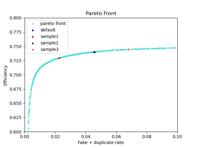
First, manually select 3 points on the pareto_front using plotting.ipynb. After you run the last cell, a file named selected_params.csv will be created in the checkpoint folder. The first row on the file corresponds to the default cuts, while the other 3 are the points you picked. The columns are the same as in pareto_front.csv, minus the last two (only the cuts are present).

To run MTV,

cd MTV
python make_plots.py   # add '-p2' for Phase-2 results