-
Notifications
You must be signed in to change notification settings - Fork 50
Bootstrap analysis
-
data from sequence alignment that capture uncertainty:
- credibility intervals for quartet concordance factors, from TICR
- bootstrap gene trees from RAxML (same format that ASTRAL uses)

-
a starting topology
Option: we can include a second network topology, to serve as the starting topology for some percentage of runs when searching for the best network, for each bootstrap replicate.
# bootstrap from bucky's credibility intervals for CFs
using CSV, DataFrames
buckyDat = CSV.read("bucky-output/1_seqgen.CFs.csv") # names like: CF12.34, CF12.34_lo etc.
rename!(buckyDat, Symbol("CF12.34") => :CF12_34)     # bootsnaq requires these colunm names
rename!(x -> Symbol(replace(String(x), "." => "_")), buckyDat) # do all in one go
bootnet = bootsnaq(net0, buckyDat, hmax=1, nrep=50, runs=3,
                   filename="snaq/bootsnaq1_buckyCI")
or
# boostrap from raxml's bootstrap gene trees
bootTrees = readBootstrapTrees("astral/BSlistfiles")
bootnet = bootsnaq(net0, bootTrees, hmax=1, nrep=50, runs=3,
                   filename="snaq/bootsnaq1_raxmlboot")
These settings are to make calculations faster. For a real data set,
up the number of bootstrap replicates to 100 or more, by changing nrep.
Also increase the number of independent search runs per replicate, runs
or just remove the runs option to get the default 10 runs.
If you close your session after having generated these bootstrap networks, you can
read them from the output file later, in a new session.
This output file ends in .out, so you would do this:
bootnet = readMultiTopology("snaq/bootsnaq1_buckyCI.out");or
bootnet = readMultiTopology("snaq/bootsnaq1_raxmlboot.out");To make summaries, it's best to re-read the reference network (best, estimated network) from file, to get a consistent numbering of nodes and edges. Here, we re-read from file, re-root the network correctly, and rotate the edges around one of the nodes to make a nicer plot like we did earlier.
net1 = readTopology("snaq/net1_bucky.out")
rootatnode!(net1, "6")
rotate!(net1, -4)To summarize the bootstrap support of the tree edges in the estimated network, we simply extract the major tree (remove all hybrid edges with γ<0.5) from the reference network and from each bootstrap network, and then count the number of times a given edge appears in the bootstrap trees.
BSe_tree, tree1 = treeEdgesBootstrap(bootnet,net1)
show(BSe_tree, allrows=true)
BSe_tree[BSe_tree[:proportion] .< 1.0, :]
where tree1 is the major tree in net1 (the best network estimated with the original data)
and BSe_tree is a data frame with the bootstrap support that each tree edge is found
in the major tree.
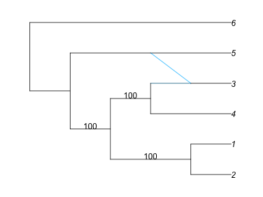
We can plot this information on the reference tree or network. The image below shows that all the tree edges in the network have 100% bootstrap support. The last command will only label the edges with bootstrap support less than 100% (if any, for other examples).
plot(tree1, :R, edgeLabel=BSe_tree);
plot(net1,  :R, edgeLabel=BSe_tree);
plot(net1,  :R, edgeLabel=BSe_tree[BSe_tree[:proportion] .< 100.0, :]);
NOTE: BSe_tree depends on edge numbers in the reference network net1,
and edge numbers change might change from session to session, depending
on how the network is obtained: output of snaq!, or read from a file.
So, you must run treeEdgesBootstrap and plot its results in the same session.
(If a network is read from a given file, its edge numbers will always be the same, though).
It is not easy to summarize bootstrap support on networks, because edges do not uniquely define splits like they do on trees. That is, it is not easy to match edges across networks.
Each hybrid node is analyzed independently of other hybridizations. That is, all other hybrid edges with γ<0.5 are removed from the network.
We focus on three types of clades:
- hybrid clade: hardwired cluster (descendants) of either hybrid edge
- major sister clade: hardwired cluster of the sibling edge of the major hybrid edge
- minor sister clade: hardwired cluster of the sibling edge of the minor hybrid edge

We compute frequencies for clades being a hybrid clade (with accompanying sister clades), and being sister clades (major or minor). The clade frequencies can be associated with a node or with an edge, and we can plot both options.
BSn, BSe, BSc, BSgam, BSedgenum = hybridBootstrapSupport(bootnet, net1);-
BSnis a table of bootstrap frequencies associated with nodes -
BSeis a table of bootstrap frequencies associated with edges, and -
BScdescribes the makeup of all clades.
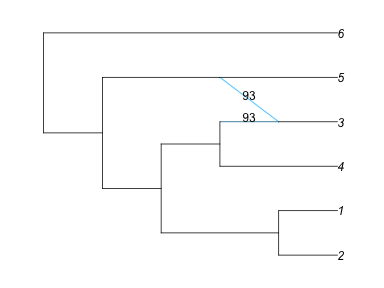
Let's go through the results step by step. We can now plot the percentage of bootstrap trees that have the same sister-hybrid relationship as in the reference network: with an edge from the same sister clade to the same hybrid clade.
plot(net1, :R, edgeLabel=BSe[[:edge,:BS_hybrid_edge]]);
It means that the 2 hybrid edges in our best network are seen in 93% of the bootstrap networks. What do the remaining 7% bootstrap networks have?
julia> BSe
8×8 DataFrames.DataFrame
│ Row │ edge    │ hybrid_clade │ hybrid  │ sister_clade │ sister │ BS_hybrid_edge │ BS_major │ BS_minor │
├─────┼─────────┼──────────────┼─────────┼──────────────┼────────┼────────────────┼──────────┼──────────┤
│ 1   │ 5       │ H7           │ 5       │ 4            │ 3      │ 93.0           │ 93.0     │ 0.0      │
│ 2   │ 9       │ H7           │ 5       │ 5            │ 7      │ 93.0           │ 0.0      │ 93.0     │
│ 3   │ missing │ c_14         │ missing │ c_minus2     │ -2     │ 3.0            │ 3.0      │ 0.0      │
│ 4   │ missing │ c_14         │ missing │ H7           │ 4      │ 3.0            │ 0.0      │ 3.0      │
│ 5   │ missing │ c_minus4     │ -4      │ c_minus2     │ -2     │ 2.0            │ 2.0      │ 0.0      │
│ 6   │ missing │ c_minus4     │ -4      │ 5            │ 7      │ 2.0            │ 0.0      │ 2.0      │
│ 7   │ missing │ 5            │ 7       │ 6            │ 6      │ 2.0            │ 2.0      │ 0.0      │
│ 8   │ missing │ 5            │ 7       │ H7           │ 4      │ 2.0            │ 0.0      │ 2.0      │
Looking at the last 2 rows, we see that 2% of the bootstrap networks have clade named "5"
(node numbered 7 in our best network) as a hybrid clade, with hybrid edges coming
from clade "6" (major sister) and from clade "H7" (minor sister).
Looking at the previous plot, this hybrid configuration is obtained by reversing the direction
of "gene flow", to occur from "3" to "5" instead "5" to "3".
Looking at rows 3 and 4, a clade named "c_14" was inferred to be a hybrid in 3% of bootstrap
replicates. What is this clade? We can see the clade membership from the table BSc:
julia> BSc
6×8 DataFrames.DataFrame
│ Row │ taxa │ 4     │ H7    │ c_minus4 │ 6     │ 5     │ c_minus2 │ c_14  │
├─────┼──────┼───────┼───────┼──────────┼───────┼───────┼──────────┼───────┤
│ 1   │ 1    │ false │ false │ false    │ false │ false │ true     │ false │
│ 2   │ 2    │ false │ false │ false    │ false │ false │ true     │ false │
│ 3   │ 4    │ true  │ false │ true     │ false │ false │ false    │ false │
│ 4   │ 3    │ false │ true  │ true     │ false │ false │ false    │ false │
│ 5   │ 6    │ false │ false │ false    │ true  │ false │ false    │ true  │
│ 6   │ 5    │ false │ false │ false    │ false │ true  │ false    │ true  │

julia> BSc[:taxa][BSc[:c_14]]
2-element DataArrays.DataArray{ASCIIString,1}:
 "6"
 "5"
Bootstrap support for the full reticulation relationships in the network, one at each hybrid node (support for same hybrid with same sister clades)
plot(net1, :R, nodeLabel=BSn[[:hybridnode,:BS_hybrid_samesisters]]);
This means that in 93% of the bootstrap networks, we have the same reticulation relationship with taxon "3" as hybrid clade, taxon "5" as one sister clade (either minor or major) and taxon "4" the other sister clade. In this example, each of these clades is made up of a single taxon, but that need not be the case in general.
We can also plot the bootstrap support for hybrid clades, regardless of their sisters. Here, it is shown on the parent edge of each node with positive hybrid support
plot(net1, :R, edgeLabel=BSn[BSn[:BS_hybrid].>0, [:edge,:BS_hybrid]]);
This means that taxon "3" is a hybrid clade in 93% of bootstrap networks; clade "3,4" is a hybrid clade in 2% of bootstrap networks, and taxon "5" in 2% of bootstrap networks. To get full information on other potential hybrid clades that do not appear as clades in the network, or on clades that appear as minor or major sisters:
julia> BSn
7×9 DataFrames.DataFrame
│ Row │ clade    │ node    │ hybridnode │ edge    │ BS_hybrid │ BS_sister │ BS_major_sister │ BS_minor_sister │ BS_hybrid_samesisters │
├─────┼──────────┼─────────┼────────────┼─────────┼───────────┼───────────┼─────────────────┼─────────────────┼───────────────────────┤
│ 1   │ H7       │ 4       │ 5          │ 4       │ 93.0      │ 5.0       │ 0.0             │ 5.0             │ 93.0                  │
│ 2   │ 5        │ 7       │ 7          │ 8       │ 2.0       │ 95.0      │ 0.0             │ 95.0            │ missing               │
│ 3   │ 4        │ 3       │ 3          │ 3       │ 0.0       │ 93.0      │ 93.0            │ 0.0             │ missing               │
│ 4   │ c_minus2 │ -2      │ -2         │ 12      │ 0.0       │ 5.0       │ 5.0             │ 0.0             │ missing               │
│ 5   │ c_14     │ missing │ missing    │ missing │ 3.0       │ 0.0       │ 0.0             │ 0.0             │ missing               │
│ 6   │ c_minus4 │ -4      │ -4         │ 6       │ 2.0       │ 0.0       │ 0.0             │ 0.0             │ missing               │
│ 7   │ 6        │ 6       │ 6          │ 7       │ 0.0       │ 2.0       │ 2.0             │ 0.0             │ missing               │
Finally, we can get information on the estimated heritabilities γ in the bootstrap network, for the replicates in which the same hybrid edges are found as in the best network:
BSgam # array of gamma values
minimum(BSgam[:,2])
maximum(BSgam[:,2])
using Statistics
mean(BSgam[:,2])
std(BSgam[:,2])
Next: formal TICR test to test a tree with ILS only.
PhyloNetworks Workshop
- home
- example data
-
TICR pipeline:
from sequences to quartet CFs
- the data
- MrBayes on all genes
- BUCKy
- Quartet MaxCut
- RAxML & ASTRAL
- PhyloNetworks: from quartet CFs or gene trees to phylogenetic networks
- TICR test: is a population tree with ILS sufficient (vs network)?
- Continuous trait evolution on a network