Welcome to stable diffusion playground! Use this repo to generate cool images!
Also - you get reproducibility for free! You'll know exactly how you created all of your images.
The metadata and latent information is stored inside of the image and into a npy file respectively.
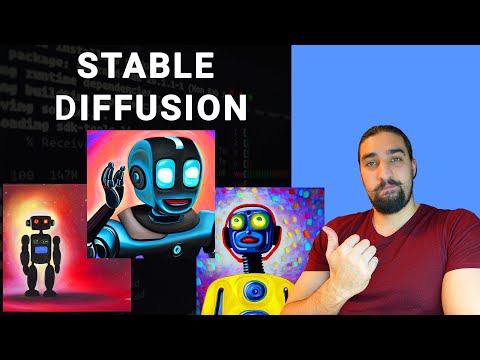
Here are some images I generated using the prompt: a painting of an ai robot having an epiphany moment:
If you generate something cool, tag me on Twitter 🐦 @gordic_aleksa - I'd love to see what you create.
Follow the next steps to run this code:
git clone https://github.com/gordicaleksa/stable_diffusion_playground- Open Anaconda console and navigate into project directory
cd path_to_repo - Run
conda env createfrom project directory (this will create a brand new conda environment). - Run
activate sd_playground(for running scripts from your console or setup the interpreter in your IDE) - Run
huggingface-cli loginbefore the first time you try to use it to access model weights.
That's it! It should work out-of-the-box executing environment.yml file which deals with dependencies.
Important note: you have to locally patch the pipeline_stable_diffusion.py file from the diffusers 0.2.4 lib
using the code from the main branch. The changes I rely (having latents as an argument) on still haven't propagated to the pip package.
The script can be run using an IDE (such as vscode, PyCharm, etc.) but it can also be run via command line thanks to fire package. fire makes things much more concise than using argparse! E.g. if there is an argument in the generate_images function with name <arg_name> then you can call python generate_images.py --<arg_name> <arg_value>.
Next up - a brief explanation of certain script arguments.
output_dir_name is the name of the output directory.
- Your images will be stored at
output/<output_dir_name>/imgs. - Your latents will be stored at
output/<output_dir_name>/latents. - Your metadata will be stored inside of the
user_commentexif tag ifsave_metadata_to_img==Trueotherwise it'll be saved tooutput/<output_dir_name>/metadata.
All of this relative to from where you're running the code.
prompt, guidance_scale, seed, num_inference_steps are the main knobs you have at your disposal to control image generation.
Check out the code comments for more info.
Finally, the script has 3 modes of execution - let me explain each of them below.
Set execution_mode=ExecutionMode.GENERATE_DIVERSE.
It will generate num_imgs images (of widthxheight resolution) and store them (as well as other info as described above) into the output file structure.
Use the main knobs as described above to control the content and quality of the image.
Here are some images I generated using this mode:
Set execution_mode=INTERPOLATE.
There are 2 ways to run this mode:
- Run
GENERATE_DIVERSEand pick the 2 images you like. Grab paths to their latents (you'll find them underoutput/<output_dir_name>/latents) and specify them inside ofsrc_latent_pathandtrg_latent_path. After this the code will spherically interpolatenum_imgsbetween them and by doing that generate a (mostly) smooth transition from source image into the target one. - Don't specify the latents - they will be generated on the fly so you won't know how your source and target image look like upfront. Everything else remains the same.
As an example I'll take the 2 images from above and interpolate between them here is the resulting grid:
Note: I generated 200 images but had to subsample to only 32 for this grid image. But in general there are always sudden jumps in the decoded image space unless you move with very fine steps through the latent space.
Set execution_mode=REPRODUCE.
This one is more for debugging purposes.
Specify src_latent_path and metadata_path. For metadata_path specify either the actual metadata .json file path or simply the image path if it contains the metadata (this depends on save_metadata_to_img flag).
After this the script will reconstruct the original image - showcasing the reproducibility.
You need a GPU that has at least 8 GBs of VRAM to run this at 512x512 in fp16 precision.
If you wish to run it in fp32 precision you will need ~16 GBs of VRAM (unless you're willing to sacrifice resolution).
fp16 flag controls whether you load the fp16 or fp32 weights.
Here is a video walk-through of this repo:
(the commit I used in the video is this one)
And here is a deep dive video going through the stable diffusion codebase:
💼 LinkedIn 🐦 Twitter 👨👩👧👦 Discord
📺 YouTube 📚 Medium 💻 GitHub 📢 AI Newsletter - one day heh
Took inspiration from Karpathy's gist.


