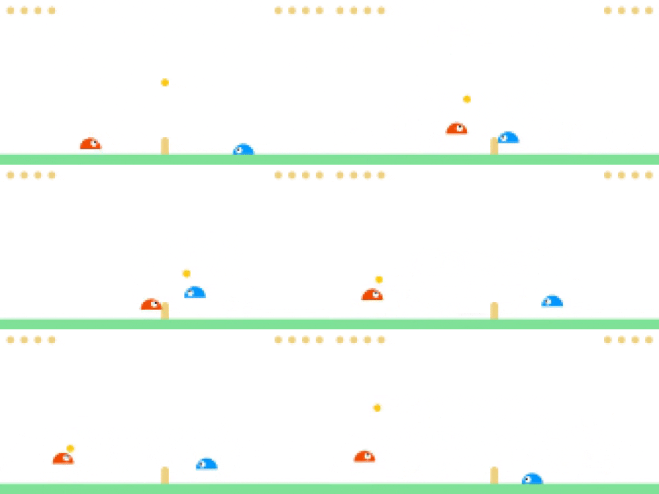
Slime Volleyball is a game created in the early 2000s by an unknown author.
“The physics of the game are a little ‘dodgy,’ but its simple gameplay made it instantly addictive.”
Update (May 12, 2022): This environment has been ported over to EvoJAX, hardware-accelerated neuroevolution toolkit that allows SlimeVolley to run on GPUs, enabling training time in minutes rather than hours.
SlimeVolleyGym is a simple gym environment for testing single and multi-agent reinforcement learning algorithms.
The game is very simple: the agent's goal is to get the ball to land on the ground of its opponent's side, causing its opponent to lose a life. Each agent starts off with five lives. The episode ends when either agent loses all five lives, or after 3000 timesteps has passed. An agent receives a reward of +1 when its opponent loses or -1 when it loses a life.
This environment is based on Neural Slime Volleyball, a JavaScript game I created in 2015 that used self-play and evolution to train a simple neural network agent to play the game better than most human players. I decided to port it over to Python as a lightweight and fast gym environment as a testbed for more advanced RL methods such as multi-agent, self-play, continual learning, and imitation learning algorithms.
-
The pre-trained PPO models were trained using stable-baselines v2.10, not stable-baselines3.
-
The examples were developed based on Gym version 0.19.0 or earlier. I tested 0.20.0 briefly and it seems to work, but later versions of Gym have API-breaking changes.
-
I used pyglet library 0.15.7 or earlier while developing this, but have not tested whether the package works for the latest versions of pyglet.
-
Only dependencies are gym and numpy. No other libraries needed to run the env, making it less likely to break.
-
In the normal single agent setting, the agent plays against a tiny 120-parameter neural network baseline agent from 2015. This opponent can easily be replaced by another policy to enable a multi-agent or self-play environment.
-
Runs at around 12.5K timesteps per second on 2015 MacBook (core i7) for state-space observations, resulting in faster iteration in experiments.
-
A tutorial demonstrating several different training methods (e.g. single agent, self-play, evolution) that require only a single CPU machine in most cases. Potentially useful for educational purposes.
-
A pixel observation mode is available. Observations are directly rendered to numpy arrays and runs on headless cloud machines. The pixel version of the environment mimics gym environments based on the Atari Learning Environment and has been tested on several Atari gym wrappers and RL models tuned for Atari.
-
The opponent's observation is made available in the optional
infoobject returned byenv.step()for both state and pixel settings. The observations are constructed as if the agent is always playing on the right court, even if it is playing on the left court, so an agent trained to play on one side can play on the other side without adjustment.
This environment is meant to complement existing simple benchmark tasks, such as CartPole, Lunar Lander, Bipedal Walker, Car Racing, and continuous control tasks (MuJoCo / PyBullet / DM Control), but with an extra game-playing element. The motivation is to easily enable trained agents to play against each other, and also let us easily train agents directly in a multi-agent setting, thus adding an extra dimension for evaluating an agent's performance.
Install from pip package, if you only want to use the gym environment, but don't want the example usage scripts:
pip install slimevolleygym
Install from the repo, if you want basic usage demos, training scripts, pre-trained models:
git clone https://github.com/hardmaru/slimevolleygym.git
cd slimevolleygym
pip install -e .
After installing from the repo, you can play the game against the baseline agent by running:
python test_state.py
You can control the agent on the right using the arrow keys, or the agent on the left using (A, W, D).
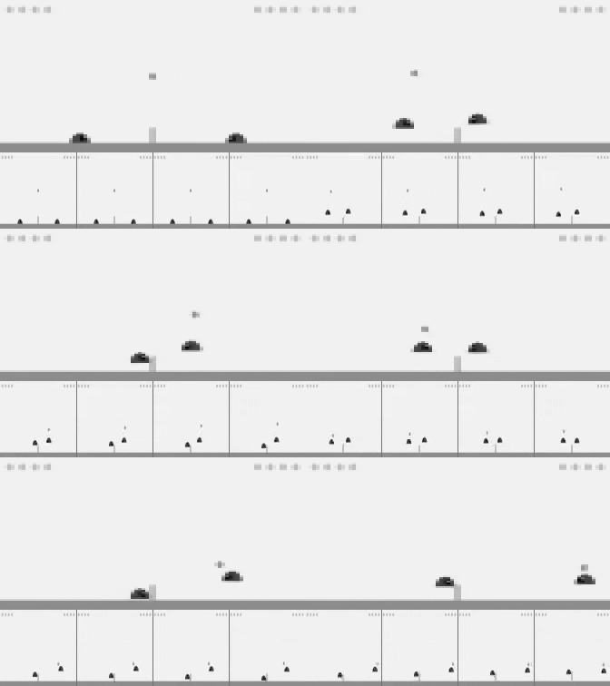
Similarly, test_pixel.py allows you to play in the pixelated environment, and test_atari.py lets you play the game by observing the preprocessed stacked frames (84px x 84px x 4 frames) typically done for Atari RL agents:

Atari gym wrappers combine 4 frames as one observation.
There are two types of environments: state-space observation or pixel observations:
| Environment Id | Observation Space | Action Space |
|---|---|---|
| SlimeVolley-v0 | Box(12) | MultiBinary(3) |
| SlimeVolleyPixel-v0 | Box(84, 168, 3) | MultiBinary(3) |
| SlimeVolleyNoFrameskip-v0 | Box(84, 168, 3) | Discrete(6) |
SlimeVolleyNoFrameskip-v0 identical to SlimeVolleyPixel-v0 except that the action space is now a one-hot vector typically used in Atari RL agents.
In state-space observation, the 12-dim vector corresponds to the following states:
The origin point (0, 0) is located at the bottom of the fence.
Both state and pixel observations are presented assuming the agent is playing on the right side of the screen.
It is straight forward to modify the gym loop to enable multi-agent or self-play. Here is a basic gym loop:
import gym
import slimevolleygym

env = gym.make("SlimeVolley-v0")

obs = env.reset()
done = False
total_reward = 0

while not done:
  action = my_policy(obs)
  obs, reward, done, info = env.step(action)
  total_reward += reward
  env.render()

print("score:", total_reward)
The info object contains extra information including the observation for the opponent:
info = {
  'ale.lives': agent's lives left,
  'ale.otherLives': opponent's lives left,
  'otherObs': opponent's observations,
  'state': agent's state (same as obs in state mode),
  'otherState': opponent's state (same as otherObs in state mode),
}
This modification allows you to evaluate policy1 against policy2
obs1 = env.reset()
obs2 = obs1 # both sides always see the same initial observation.

done = False
total_reward = 0

while not done:

  action1 = policy1(obs1)
  action2 = policy2(obs2)

  obs1, reward, done, info = env.step(action1, action2) # extra argument
  obs2 = info['otherObs']

  total_reward += reward
  env.render()

print("policy1's score:", total_reward)
print("policy2's score:", -total_reward)
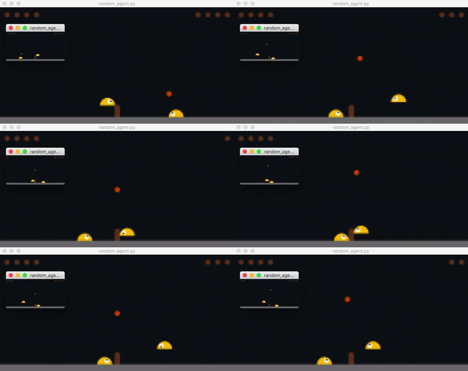
Note that in both state and pixel modes, otherObs is given as if the agent is playing on the right side of the screen, so one can swap an agent to play either side without modifying the agent.

Opponent's observation is rendered in the smaller window.
One can consider replacing policy2 with earlier versions of your agent (self-play) and wrapping the multi-agent environment as if it were a single-agent environment so that it can use standard RL algorithms. There are several examples of these techniques described in more detail in the TRAINING.md tutorial.
Several pre-trained agents (ppo, cma, ga, baseline) are discussed in the TRAINING.md tutorial.
You can run them against each other using the following command:
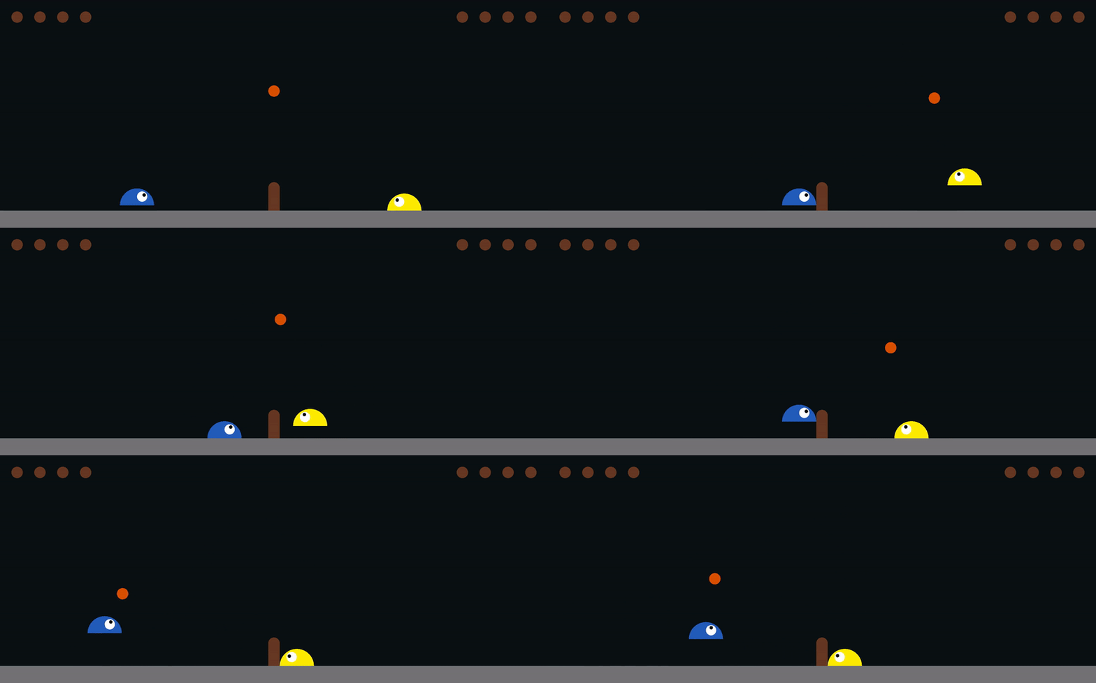
python eval_agents.py --left ppo --right cma --render

Evaluating PPO agent (left) against CMA-ES (right).
It should be relatively straightforward to modify eval_agents.py to include your custom agent.
Below are scores achieved by various algorithms and links to their implementations. Feel free to add yours here:
| Method | Average Score | Episodes | Other Info |
|---|---|---|---|
| Maximum Possible Score | 5.0 | ||
| PPO | 1.377 ± 1.133 | 1000 | link |
| CMA-ES | 1.148 ± 1.071 | 1000 | link |
| GA (Self-Play) | 0.353 ± 0.728 | 1000 | link |
| CMA-ES (Self-Play) | -0.071 ± 0.827 | 1000 | link |
| PPO (Self-Play) | -0.371 ± 1.085 | 1000 | link |
| Random Policy | -4.866 ± 0.372 | 1000 | |
| Add Method |
For sample efficiency, we can measure how many timesteps it took to train an agent that can achieve a positive average score (over 1000 episodes) against the built-in baseline policy:
| Method | Timesteps (Best) | Timesteps (Median) | Trials | Other Info |
|---|---|---|---|---|
| PPO | 1.274M | 2.998M | 17 | link |
| Data-efficient Rainbow | 0.750M | 0.751M | 3 | link |
| Add Method |
Table of average scores achieved versus agents other than the default baseline policy (1000 episodes):
| Method | Baseline | PPO | CMA-ES | GA (Self-Play) | Other Info |
|---|---|---|---|---|---|
| PPO | 1.377 ± 1.133 | — | 0.133 ± 0.414 | -3.128 ± 1.509 | link |
| CMA-ES | 1.148 ± 1.071 | -0.133 ± 0.414 | — | -0.301 ± 0.618 | link |
| GA (Self-Play) | 0.353 ± 0.728 | 3.128 ± 1.509 | 0.301 ± 0.618 | — | link |
| CMA-ES (Self-Play) | -0.071 ± 0.827 | -0.749 ± 0.846 | -0.351 ± 0.651 | -4.923 ± 0.342 | link |
| PPO (Self-Play) | -0.371 ± 1.085 | 0.119 ± 1.46 | -2.304 ± 1.392 | -0.42 ± 0.717 | link |
| Add Method |
It is interesting to note that while GA (Self-Play) did not perform as well against the baseline policy compared to PPO and CMA-ES, it is a superior policy if evaluated against these methods that trained directly against the baseline policy.
Results for pixel observation version of the environment (SlimeVolleyPixel-v0 or SlimeVolleyNoFrameskip-v0):
| Pixel Observation | Average Score | Episodes | Other Info |
|---|---|---|---|
| Maximum Possible Score | 5.0 | ||
| PPO | 0.435 ± 0.961 | 1000 | link |
| Rainbow | 0.037 ± 0.994 | 1000 | link |
| A2C | -0.079 ± 1.091 | 1000 | link |
| ACKTR | -1.183 ± 1.480 | 1000 | link |
| ACER | -1.789 ± 1.632 | 1000 | link |
| DQN | -4.091 ± 1.242 | 1000 | link |
| Random Policy | -4.866 ± 0.372 | 1000 | |
| Add Method | (>= 1000) |
If you have publications, articles, projects, blog posts that use this environment, feel free to add a link here via a PR.
Please use this BibTeX to cite this repository in your publications:
@misc{slimevolleygym,
  author = {David Ha},
  title = {Slime Volleyball Gym Environment},
  year = {2020},
  publisher = {GitHub},
  journal = {GitHub repository},
  howpublished = {\url{https://github.com/hardmaru/slimevolleygym}},
}
