Decision trees are non-parametric supervised learning algorithms (for both classification and regression) that tries to model the problems without any assumptions on data (unlike logistic regression, linear regression etc). AT each step, decision tree asks a binary question for all feature-value pair and select best question that yield best separation based on decision criteria (Gini impurity or information gain in the case of classification problem and MSE or MAE in the case of regression problem).
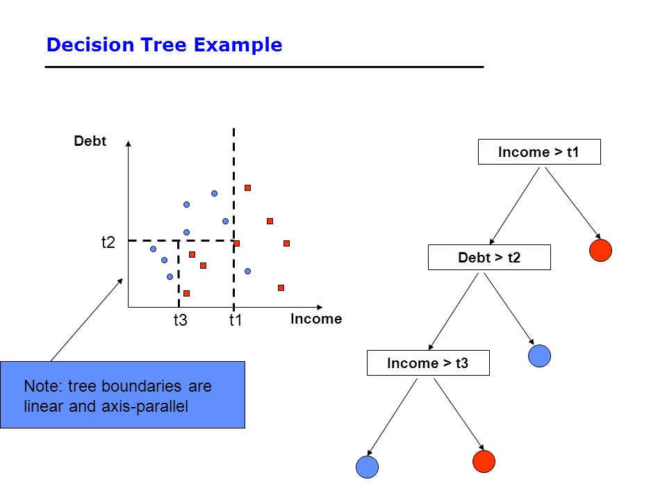
Geometrically it tries to divide the feature space into two half at each iteration based on the binary questions. Programmatically Decision tree is nested if else statement, Geometrically Decision tree is set of axis parallel hyperplane.
Decision tree as axis parallel hyperplane and nested if else condition:
Decision tree geometrically and programaticallyEntropy is the measure of disorderness (or roughly can be thought of "spread"). More spread things are, more entropy (uncertainty) value it would have.
We use entropy in machine learning to find what features reduces the entropy (to find the best split in the decision tree algorithm). Entropy can range from [0, 1] for binary class settings and [0, inf] for multi class settings.
Probabilistically, entropy is measure of uncertainty, where high value denotes events are equally probable (close to uniform distribution) and low value denotes events are certain to happen
When entropy is at it's highest at that point you may assume all the values (labels) are equally likely, you don't have no information about the certainty of a particular class.
Here is the best example to understand entropy:
Uniform distribution (high entropy) and Normali distribution (low entropy)If you look at the above two distribution, which one has high entropy? Distribution which doesn't favour a particular (or set of) outcome has the high entropy, because the outcome is hard to guess. Imagine throwing a fair dice
In the cause of bell curve, we know "mean" has the most favourable outcome, so we can easily guess what would be the outcome (with high probability) if we sample from this distribution, it has low entropy. Image throwing a biased dice where number 3 shows up 50% of the time.
Formula of entropy:
Entropy equation (*Note: -log(x)= 1/x)we compute entropy for each class and sum them up to get the total entropy. Entropy will be at maximum when all the classes are equally likely. For multi class settings, entropy can approach +infinity (any value).
Plot of entropy (*binary case):
Entropy plot for binary case settingsNote how entropy is at maximum (1) when both the class are equally likely (50% chance).
- Entropy is measure of disorderness/ spread/ uncertainty.
- It's value ranges from
[0, 1], 0 being certain and 1 being uncertain for binary classification (50% chance.) - For multi class settings, It's value could be between
[0, inf]
Gini impurity (alternative to entropy because computing log is expensive than computing square of probabilities)
Gini impurity measures the uncertainty (just like entropy). It measure the probability of misclassification if an object is randomly chosen (how uncertain it is).
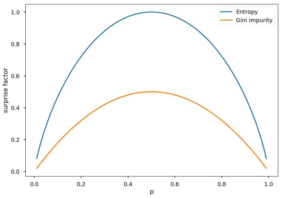
Gini Index and Entropy, Impurity Criterion Values Gini Index And Cross Entropy Can TakeNotice the maximum value of gini impurity is 0.5 while entropy's is 1 for binary case setting.
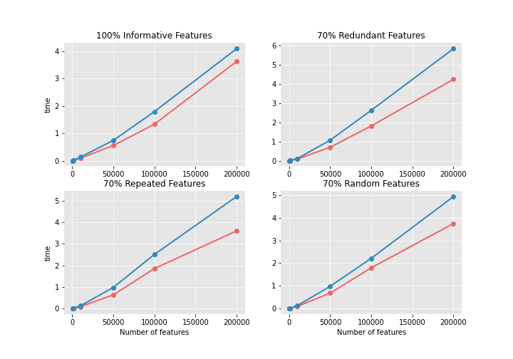
In the following graphs, the x-axis is the number of samples of the dataset and the y-axis is the training time.

As can be seen, the training time when using the Entropy criterion is much higher. Furthermore, the impact of the nature of the features is quite noticeable. Redundant features are the most affected ones, making the training time 50% longer than when using informative features. Whereas, the use of random features or repeated features have a similar impact. The differences in training time are more noticeable in larger datasets.
Decision Trees: Gini vs Entropy
- It is alternative to entropy (because entropy is computationally expensive due to log operation) and is faster to compute.
- Gini impurity is 0 if there is no uncertainty, and 0.5 when each object is equal probable (*for binary classification)
- For multi class classification Gini impurity ranges from [0, 1] rather than [0, 0.5] Calculating Gini Impurity Example
- Node with Gini impurity of 0 is called pure node because there is no ambiguity between classes
Information gain is a metric to measure how much information we are gaining after we split the data using feature-label pair. We select feature value which yields maximum information gain. Here is how Information gain is calculated:
Information Gain expressionInformation gain is calculated as : Impurity of parent node - weighted sum of child nodes.
As you can in the above tree, at the root node, we compute impurity using 1- sum of probability squared for each class. In this case, 1 - (2/5*2/5(apple) + 2/5*2/5(grape) + 1/5 * 1/5 (lemon)) = 0.64.
Once we get the root node, we compute impurity for all feature -value pair, like color= green?, color= red? and so on. We choose feature with minimum impurity, in this case the feature-value pair is is color green? which yields 0.62 gini impurity in the left subtree and 0 impurity in right subtree.
Finally we compute the information gain by taking difference between impurity in parent node and weighted impurity sum in child nodes.
ID3(creates multiway tree) Iterative Dichotomizer, was the first of three Decision Tree implementations developed by Ross Quinlan
It builds a decision tree for the given data in a top-down fashion, starting from a set of objects and a specification of properties Resources and Information. each node of the tree, one property is tested based on maximizing information gain and minimizing entropy, and the results are used to split the object set. This process is recursively done until the set in a given sub-tree is homogeneous (i.e. it contains objects belonging to the same category). The ID3 algorithm uses a greedy search. It selects a test using the information gain criterion, and then never explores the possibility of alternate choices.
Disadvantages Only one attribute at a time is tested for making a decision. Does not handle numeric attributes and missing values.
C4.5 (extension to ID3 with capability of handling numerical values as well) Improved version on ID 3 by Quinlan's. The new features (versus ID3) are: (i) accepts both continuous and discrete features; (ii) handles incomplete data points; (iii) solves over-fitting problem by (very clever) bottom-up technique usually known as "pruning"; and (iv) different weights can be applied to the features that comprise the training data.
Disadvantages
C4.5 constructs empty branches with zero values Over fitting happens when algorithm model picks up data with uncommon characteristics , especially when data is noisy.
CART (creates binary tree and handles numerical values as well)
CART stands for Classification and Regression Trees. It is characterized by the fact that it constructs binary trees, namely each internal node has exactly two outgoing edges. The splits are selected using the towing criteria and the obtained tree is pruned by cost–complexity Pruning. CART can handle both numeric and categorical variables and it can easily handle outliers.
Disadvantages
It can split on only one variable Trees formed may be unstable
- First step is to select a feature to represent the root node, This is done by computing Gini impurity or entropy on whole dataset target - weighted sum of Gini impurity of corresponding left and right child. (This simply mean, how much information we are gaining by splitting the data on a particular feature) (How much uncertainty we are reducing by splitting on a particular feature)
- Compute IG for each feature value and for all the features
- Choose feature with highest information gain and split the data
- If node is pure (contains only one class or impurity is zero), we stop and pure node becomes leaf node.
- Else we repeat this whole process and keep dividing the tree.
Process for creating regression tree is same as creating classification tree, with the change in decision criteria. Rather than using information gain, we use MSE or MAE as a decision criteria.
Decision trees are prone to overfit if they are too deep (each point is a leaf node). Underfitting is when you have too shallow tree ("a decision stump" which is tree with depth one). Bias variance trade off is controlled by many hyper parameter value, to list few of them,depth of the tree (max_depth) and number of points require to make a split (min_sample_split), minimum number of points require in the leaf node (min_samples_leaf) and so on.
Overfitting in decision tree
Overfitting in decision tree regressionGeometrically, underfitting is when you have few space partitions (axis parallel lines) and overfitting is when you have too many partitions that each data point is in own space
Training time complexity is (N * log(N) * D) + O(N * D) (assuming all the features to be numeric) where N is the number of data points (N * log(N)) for sorting, and D is number of data dimensions.
For each node, we need to perform sorting, for each sorted feature, we need to compute Gini impurity and information gain which takes (N * log(N) * D) + O(N * D) per node.
Space complexity We just need to store number of nodes in the memory. So space complexity is O(# of nodes).
Runtime complexity isO(depth of the tree), we are going to reduce the search complexity by half on each depth.
- Simple to understand and to interpret (Trees can be visualized)
- Requires little data preparation. Other techniques often require data normalization, dummy variables need to be created and blank values to be removed.
- The cost of using the tree (prediction on query point) is logarithmic in the number of data points used to train the tree
- Able to handle both numerical and categorical data. Other techniques are usually specialized in analysing datasets that have only one type of variable.
- Able to handle multi-output problems.
- Uses a white box model. If a given situation is observable in a model, the explanation for the condition is easily explained by Boolean logic. By contrast, in a black box model (in an artificial neural network for instance), results may be more difficult to interpret.
- Possible to validate a model using statistical tests. That makes it possible to account for the reliability of the model.
- Performs well even if its assumptions are somewhat violated by the true model from which the data were generated.
- Decision-tree learners can create over-complex trees that do not generalise the data well. This is called overfitting. Mechanisms such as pruning, setting the minimum number of samples required at a leaf node or setting the maximum depth of the tree are necessary to avoid this problem.
- Decision trees can be unstable because small variations in the data might result in a completely different tree being generated. This problem is mitigated by using decision trees within an ensemble.
- The problem of learning an optimal decision tree is known to be NP-complete under several aspects of optimality and even for simple concepts. Consequently, practical decision-tree learning algorithms are based on heuristic algorithms such as the greedy algorithm where locally optimal decisions are made at each node. Such algorithms cannot guarantee to return the globally optimal decision tree. This can be mitigated by training multiple trees in an ensemble learner, where the features and samples are randomly sampled with replacement.
- There are concepts that are hard to learn because decision trees do not express them easily, such as XOR, parity or multiplexer problems.
- Decision tree learners create biased trees if some classes dominate. It is therefore recommended to balance the dataset prior to fitting with the decision tree.
- As Decision tree is non-parametric it makes no assumption about the distribution of data to model the problem.
- It is a Supervised learning algorithm which partitions data on every iteration, It is a greedy algorithm.
- Geometrically hyper plains are axis parallel and non linear.
- Works great on non-linear data as well.
- It's structure is tree like data structure.
- Makes decision (make split) at ever node using gini impurity or entropy score/ MAE or MSE.
- Can be written in if else statement which mean it has low execution time and hence can be used for low latency applications.
- Highly interpretable (if else statements are easy to interpret) and visualize.
- Does not require feature standardization unlike logistic regression, SVM, KNN which are distance based method as decision tree is based on ordering of data.
- It is not a distance based method (and hence feature standardization and normalization has no effect).
- Increase in depth of tree results in overfit, it also reduce interpretability of model (many nested if else are hard to interpret) likewise decreasing depth of the tree results in underfitting.
- Robust to outliers (tree based methods are not get effected by extreme values as long as tree depth is under control).
- It can be used to solve classification as well as regression problem.
- If categorical values are huge (like pin code )convert categorical values to numeric values using technique such as response encoding could help.
- Works well even when the training data is huge and dimensionality is low.
- Balance the data if dataset is imbalanced because, Imbalance data will effect the entropy calculations because it is based on probabilities which again is based on class counts.
- Decision tree cannot work with similarity matrix unlike logistic regression or SVM (distance based classifier).
- Can do multi-class classification (as entropy and Gini impurity will take care of it).
- Decision Trees does not work well with One hot encoded features, Large dimensional data and categorical features which have large categories (we may use response encoding to get away with large categories values).
A Simple Explanation of Gini Impurity
Decision Trees: Gini vs Entropy


