-
Notifications
You must be signed in to change notification settings - Fork 293
Training Audio Models using Azure ML
Recently I posted a bunch of new Audio Keyword Spotting models that dramatically improved our pareto curve. The following chart shows by just how much, the old gallery models are marked with orange square and cyan plus, the new models are much faster and more accurate:
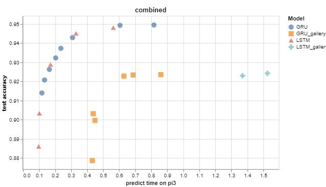
These models were found by doing quite a few parameter sweeps on Azure ML with Pytorch on a GPU cluster. A batch of 20 new models could be trained this way in just a few minutes. The hyper-parameters explored included type of PyTorch optimizer, learning rate, learning rate schedulers, weight decay, batch size, hidden size, and number of layers in the model. All in all over 500 new models were trained which were then tested on our Raspberry Pi Cluster. This revealed a nice new pareto curve and 13 all new models for our gallery.
On the bottom left of this curve are 1-layer LSTM models with small size (50 hidden units), this makes them fast at around 0.1 ms on a Raspberry Pi. In the middle are the 2-layer models which are a mix of GRU and LSTM models with hidden sizes from 80 to 110. At the top end with accuracy up around 95% are the 3-layer LSTM and GRU models that have a hidden size up to 150. We could go larger of course, but we wanted to constrain this search to those models that will fit on the Azure IoT DevKit which has an ARM Cortex-M4f CPU with 1mb flash and 256kb RAM.
All this shows that if you train enough models with enough variation in parameters you can fill in a very smooth convex pareto curve. This provides the best set of models for you to choose from base on your application's requirements, trading off between speed and accuracy.
I found the best way to manage all this was to do the following:
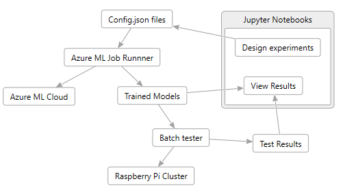
I used Jupyter Notebooks to "design" the experiments. This notebook would just write out a folder for each experiment and each of these experiments contained subfolders for each job, which was described by a json config file. Each experiment represented a specific parameter sweep with somewhere between 10 and 20 models each. Then I wrote an Azure ML "runner" python script which would monitor these folders for new work, send those jobs to Azure ML, and download the results when the jobs were finished.
Then I used some other Jupyter Notebooks with VegaLite to plot the training results, learning rates, and so on, so I could check the training results, fine tune parameters, submit more experiments and so forth. By the time I was done I had probably thrown away half of the experiments I designed. It is an iterative job.
Once I had a bunch of good models I was ready to run my batch_test.py script to test the models. This involes importing the models from ONNX into the ELL format, compiling them with the ELL wrap tool, running them on our Raspberry Pi Cluster with a small test set to measure performance, and then running them again on my PC with the full test set to make sure the test accuracy of the compiled ELL models matches the test accuracy reported by PyTorch. I'm happy to report the accuracy was very close, usually within 0.1%.
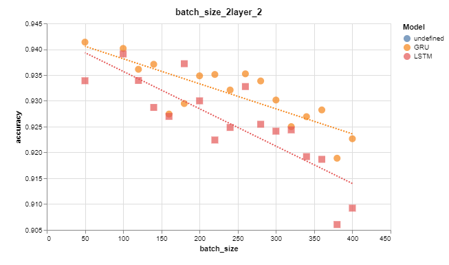
Here's a few plots to give you an idea of the sort of thing I was looking for. In this first one we see that batch size has a negative impact on accuracy:
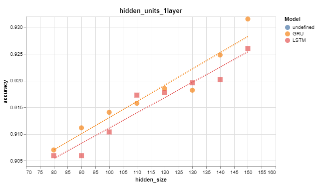
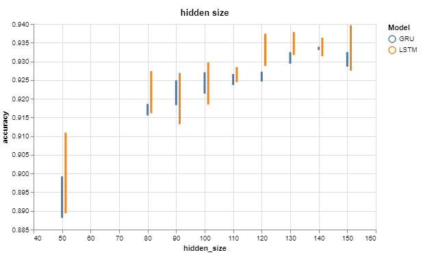
Conversely, the number of hidden units on the RNN node directly improves accuracy:
Similarly, I wanted to see how much variation there is in accuracy when I run multiple identical experiments, this graph shows there is quite a bit of variation, perhaps more for smaller models. But the trend is still clearly upwards:
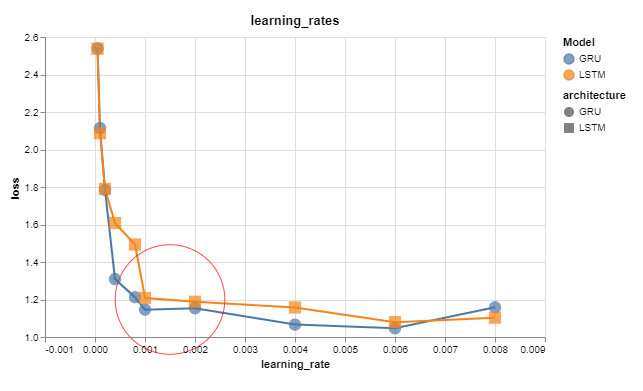
When finding the right range of learning rates it is useful to plot the training loss against the learning rate and I found this:
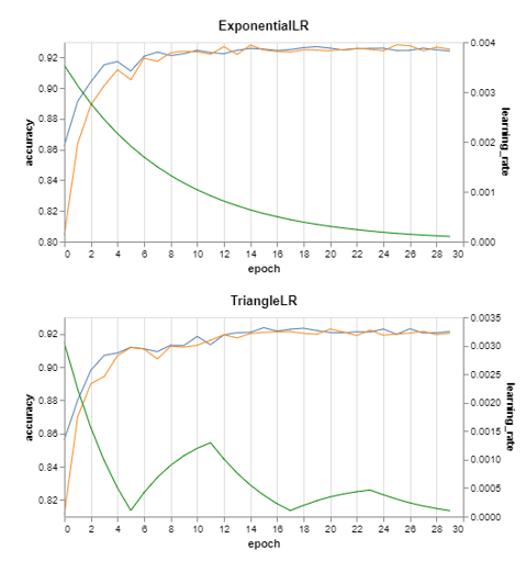
When searching different learning rate schedulers, it was useful to plot the accuracy with the actual learning rate:
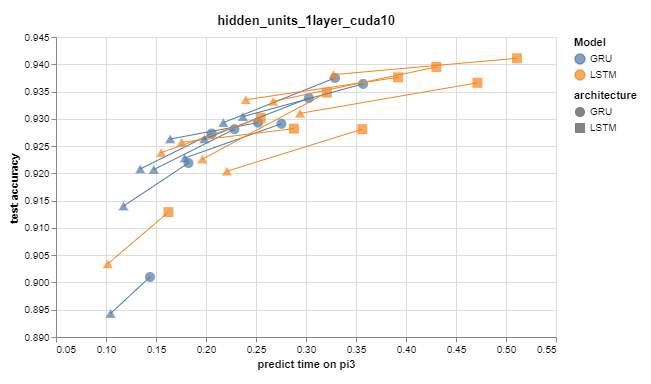
When it came time to look at the test accuracy versus the predict time, I also wanted to see the performance impact of using "HardSigmoid" instead of the more expensive "Sigmoid" and these arrows show the result. Hard Sigmoid is faster, but less accurate, and the accuracy impact is higher for smaller models.
And of course it is fun to look at all 500 models to see how they stack up against each other. Clearly there's a lot of models that are not any good, in fact 13/500 is only 2.6% of models made it through the process to the model gallery.
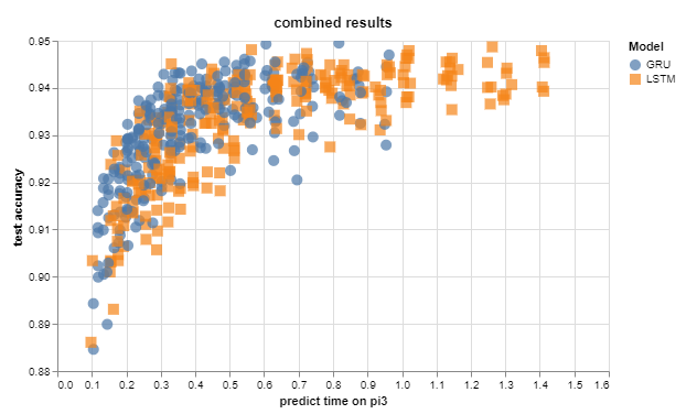
Then it is a simple matter of running a convex pareto algorithm over this result to get the new gallery models shown at the beginning of this post.
All up I found Azure ML a pleasure to work with and the quick turn around on experiments was definitely conducive to making rapid progress in the search for the best possible models.