-
Notifications
You must be signed in to change notification settings - Fork 48
TaylorGreen
Taylor flow is a two-dimensional analytical solution to the Navier-Stokes equations. The domain is [0, 2] x [0, 2] and the solution is periodic in both x- and y-directions. An interesting feature of the Taylor Green solution is that the pressure and convective terms exactly balance leaving a viscous decay of the initial solution. The analytical velocities and pressure are given at all times as

where 
To implement the Taylor Green problem we need to initialize the solution and set up the periodic boundary conditions. The entire problem file TaylorGreen2D.py reads:
from ..NSfracStep import *

# Return a mesh here. If mesh is a callable function, then you may overload its parameters.
def mesh(Nx, Ny, **params):
    return RectangleMesh(0, 0, 2, 2, Nx, Ny)

# Override some problem specific parameters
NS_parameters.update(
    nu = 0.01,         # Kinematic viscosity
    T = 1,             # End time
    dt = 0.001,        # Timestep
    Nx = 20, Ny=20,    # Mesh size
    folder = "taylorgreen2D_results",  # folder for storing results
    checkpoint = 1000, # Overwrite solution in Checkpoint folder each checkpoint tstep
    save_step = 10,    # Store solution in new folder each save_step tstep
    max_iter = 1,      # Number of velocity/pressure iterations on each timestep
    use_krylov_solvers = False,
    compute_error = 1,
    velocity_degree = 1,
    pressure_degree = 1
)

class PeriodicDomain(SubDomain):

    def inside(self, x, on_boundary):
        # True if on left or bottom boundary AND NOT on one of the two corners (0, 1) and (1, 0)
        return bool((near(x[0], 0) or near(x[1], 0)) and
              (not ((near(x[0], 0) and near(x[1], 2)) or
                    (near(x[0], 2) and near(x[1], 0)))) and on_boundary)

    def map(self, x, y):
        if near(x[0], 2) and near(x[1], 2):
            y[0] = x[0] - 2.0
            y[1] = x[1] - 2.0
        elif near(x[0], 2):
            y[0] = x[0] - 2.0
            y[1] = x[1]
        else:
            y[0] = x[0]
            y[1] = x[1] - 2.0

constrained_domain = PeriodicDomain()

initial_fields = dict(
    u0='-sin(pi*x[1])*cos(pi*x[0])*exp(-2.*pi*pi*nu*t)',
    u1='sin(pi*x[0])*cos(pi*x[1])*exp(-2.*pi*pi*nu*t)',
    p='-(cos(2*pi*x[0])+cos(2*pi*x[1]))*exp(-4.*pi*pi*nu*t)/4.')

def initialize(q_, q_1, q_2, VV, t, nu, dt, **NS_namespace):
    """Initialize solution.

    Use t=dt/2 for pressure since pressure is computed in between timesteps.

    """
    for ui in q_:
        deltat = dt/2. if ui is 'p' else 0.
        vv = project(Expression((initial_fields[ui]), t=t+deltat, nu=nu), VV[ui])
        q_[ui].vector()[:] = vv.vector()[:]
        if not ui == 'p':
            q_1[ui].vector()[:] = q_[ui].vector()[:]
            q_2[ui].vector()[:] = q_[ui].vector()[:]

def temporal_hook(q_, t, nu, VV, dt, plot_interval, initial_fields, tstep, sys_comp,
                  compute_error, **NS_namespace):
    """Function called at end of timestep.

    Plot solution and compute error by comparing to analytical solution.
    Remember pressure is computed in between timesteps.

    """
    if tstep % plot_interval == 0:
        plot(q_['u0'], title='u')
        plot(q_['u1'], title='v')
        plot(q_['p'], title='p')
    if tstep % compute_error == 0:
        err = {}
        for i, ui in enumerate(sys_comp):
            deltat_ = dt/2. if ui is 'p' else 0.
            ue = Expression((initial_fields[ui]), t=t-deltat_, nu=nu)
            ue = interpolate(ue, VV[ui])
            uen = norm(ue.vector())
            ue.vector().axpy(-1, q_[ui].vector())
            error = norm(ue.vector())/uen
            err[ui] = "{0:2.6e}".format(norm(ue.vector()))
            total_error[i] += error*dt
        print "Error is ", err, " at time = ", t
Note that this module contains one mesh and one dictionary called NS_parameters. These are required by the Navier Stokes solver. There are more default parameters found in the problems/NSfracStep/__init__.py file. A solution that can be used for visualization will be saved every 10'th timestep (the save_step parameter) to a folder called taylorgreen2D_results/Timeseries. There is also the possibility to store intermediate solutions to a Checkpoint folder. Here we store two previous timesteps of the solution vector and as such the solution can be used to obtain a clean restart (since two previous timesteps are required for the convection term). The solution in the Checkpoint folder is owerwritten continuously, so only the save_step option should be used to create animations etc. The solution is always stored together with the NS_parameters dictionary to allow for clean restarts and to remember solution parameters, like timestep, viscosity etc.
The module also contains a SubDomain named constrained_domain that sets up the two periodic directions. The remaining code is initialization and a function called temporal_hook that is called at the end of each timestep. Here we choose to plot the solution and print out the error by comparing to the analytical solution.
Running the solver in IPython is accomplished as:
>>> oasis NSfracStep problem=TaylorGreen2D Nx=100 Ny=100
Start simulations
Error is  {'p': '2.169978e-05', 'u1': '1.171413e-05', 'u0': '1.171413e-05'}  at time =  0.001
Error is  {'p': '2.536549e-05', 'u1': '2.338315e-05', 'u0': '2.338315e-05'}  at time =  0.002
Error is  {'p': '6.893817e-06', 'u1': '3.504730e-05', 'u0': '3.504730e-05'}  at time =  0.003
Error is  {'p': '1.029365e-05', 'u1': '4.670687e-05', 'u0': '4.670687e-05'}  at time =  0.004
Error is  {'p': '1.875239e-05', 'u1': '5.836182e-05', 'u0': '5.836182e-05'}  at time =  0.005
Error is  {'p': '2.800661e-05', 'u1': '7.001213e-05', 'u0': '7.001213e-05'}  at time =  0.006
Error is  {'p': '3.746201e-05', 'u1': '8.165781e-05', 'u0': '8.165781e-05'}  at time =  0.007
Error is  {'p': '4.699257e-05', 'u1': '9.329887e-05', 'u0': '9.329887e-05'}  at time =  0.008
Error is  {'p': '5.655644e-05', 'u1': '1.049353e-04', 'u0': '1.049353e-04'}  at time =  0.009
Error is  {'p': '6.613584e-05', 'u1': '1.165671e-04', 'u0': '1.165671e-04'}  at time =  0.01
...
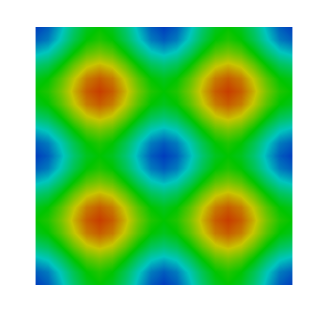
The pressure solution plotted in ParaView should look something like:

You may now experiment with higher order elements, shorter timesteps or more velocity/pressure iterations on each timestep.