Final project repository for ECSE 415, Fall 2018
Shawn Vosburg
Tristan Bouchard
Alex Masciotra
Nayem Alam
Thomas Philippon
Babatunde Onadipe
https://towardsdatascience.com/detecting-vehicles-using-machine-learning-and-computer-vision-e319ee149e10 (great article)
https://github.com/bdjukic/CarND-Vehicle-Detection (the author of the previous article's github)
ECSE415 – Intro to Computer Vision
| Name | ID |
|---|---|
| Nayem Alam | 260743549 |
| Tristan Bouchard | 260747124 |
| Alex Masciotra | 260746829 |
| Thomas Philippon | 260747645 |
| Shawn Vosburg | 260743167 |
The final project allowed us to learn and implement machine-learning related algorithms to analyze a specific dataset. The two problems that were addressed are classification and localization. The classification task required us to extract features to classify the type of object within an image. The localization task required us to pick objects of interest from a large image to classify them. The tools used in this project were a Jupyter Notebook with python3 programming language, and the MIO-TCD image dataset.
The purpose of this project was given to exercise the skills acquired from previous assignments to building a classification system using several algorithms, namely the SVM & K-Nearest-Neighbor classifier. The reason why these two methods were selected was because SVM was required by the project document & K-Nearest-Neighbor was implemented due to its simplicity. In order to initiate the project, students were paired in groups of 4-5, provided a source for acquiring a dataset [1] and implemented code within an open-source web application, Jupyter. Students were given 3 weeks to complete this project.
The dataset that was used is called the MIO-TCD-Classification set [1]. The dataset originally contained 519,194 training images, that were a part of 11 categories. These categories are different types of vehicles and modes of transportation, such as: 10,346 samples of an articulated truck, 5120 samples of a single-unit truck, 50,906 samples of a pickup truck, 10,316 samples of a bus, 260,518 samples of a car, 1982 samples of a motorcycle, 9679 samples of a work van, 2284 samples of a bicycle, 1751 samples of non-motorized vehicles, 6292 samples of pedestrian and 160, 000 samples of backgrounds.
However, we decided to select 2200 samples of each of the categories and selected all the samples for every category that contained less than 2200, in total we have 23,533 samples. This choice was made because it’s large enough to acquire enough details but not large enough to prolong runtime. Moreover, all the images were resized to dimensions of 128x128 pixels for them to all be uniformized as it helped in optimizing the code.
The extracted features were the gradients of the images and these features were extracted using the Histogram of Oriented Gradient (HoG) feature descriptor to train our SVM and K-Nearest-Neighbor (KNN). This feature was chosen because it’s amongst one of the most popular object detectors [3], it provides a compressed and encoded version of our images while also maintaining the general shape of the object. The HoG method investigates the gradients in several different directions to then computing a histogram of the resulting gradient change.
In order to detect precise edges within images, the feature extraction hyperparameters that were used were a cell size of 8x8 pixels, block size with 2x2 cells, and 8 angular directions (every 45 along a unit circle). Since our images are 128x128 pixels, our features size is 16x16x8 which is 2048 dimensions. These parameters were used because they provide sharp HoG features while keeping the size of the features low. We selected 8 directions because it generalizes every direction appropriately without the gradients being repetitive.
There were different types of vehicles, meaning the training images were not consistent, such as the backgrounds weren’t consistent, and the pixel intensities weren’t consistent. However, the general shapes remained consistent, for example, the shape of a bicycle resembles a bicycle but not the shape of a car. Hence, the HoG descriptor suited the needs for this criterion. A sample of our HoG feature extractor can be found on Appendix I.
We used the Support Vector Machine (SVM) classifier. In brief, this algorithm takes labelled training data and outputs an optimal hyperplane separating classes [2]. The SVM was implemented using the scikit-learn library (machine learning library). Three important parameters to the SVM are the kernel type, gamma, and penalty parameter C.
The kernel calculates the distance between features on an image. The kernel type that was chosen was the Radial Basis Function (RBF), in order to measure the similarity between two sets of features. RBF basis its distance between two features exponentially, which allows for quick computation. Initially we considered another kernel type, linear, but its computation time took about two times more than the RBF kernel type which means that this increases the cost of doing validation. Also, since backgrounds contain a lot of noise, our dataset is not distributed linearly.
The gamma parameter defines how far the influence of a single training example reaches; if gamma has a low value, this means that every point has a further reach. Conversely, if gamma has a high value, this means that each training example has a closer reach [4]. This parameter was set to 1/n where n is the number of features. We chose to do this because we wanted gamma to be small in order to make the training data have the largest radius of influence, since the images were noisy to begin with.
The penalty parameter C describes the margin of error of the classifier (SVM). A higher C would entail a smaller margin of error in building the classifier, however, this would result in a higher runtime. Since our images were significantly noisy, we wanted a very small margin of error, thus we set C to 100.
KNN was also acquired from the scikit-learn library and it calculates the label of its nearest neighbors while determining the mode of their labels. We used KNN due to its simplicity and its rapid building/predicting time. The parameter of KNN is the number of neighbors (n_neighbors) it observes to make a prediction. We selected 3 as the number of nearest neighbors, keeping the search radius small. Initially we tried with n_neighbors = 11 (the number of categories), but for the categories that have lower number of data points (e.g. motorcycle), it would often get misclassified as a part of a category with more data points (e.g. background).
In order to evaluate our classifiers, we used k-fold cross-validation which is dividing up our dataset into two sets, a training and a test set. The process is ideally dividing up a part of the dataset into 10 bins; 9 out of 10 are used as training and the remaining 1 is used as a test set. This process is repeated such that every bin is used as a test set once.
We performed k-fold cross validation by first randomizing the features’ order such that each bin contains about the same number of images of each category/label. Then a classifier (KNN or SVM) was trained with the k-fold cross validation process. By following this approach, it gave us a good idea of how the main classifiers, trained with all images in the dataset, will label images that were not initially available to them during training.
To evaluate the performance, the following metrics were obtained: the average classification accuracy, precision and recall across validations including standard deviations can be found on Table I.
Classification Metrics
| Classifiers | Accuracy | Standard dev. | Precision | Recall |
|---|---|---|---|---|
| SVM | 0.93677 | 0.00812 | 0.65053 | 0.64953 |
| KNN | 0.94658 | 0.01412 | 0.72876 | 0.70371 |
Average classification accuracy across validations; standard deviation, precision and recall
Notice, the precision and recall values are not consistent with accuracy because they are not evaluating the same statistics. Accuracy returns the percentage of true positives and true negatives of every prediction. As an example, this means that a car label that is actually a bicycle will return a true negative for a bus, driving up the accuracy percentage. The accuracy metric is erroneous since we can only return one label at a time. That is, for every bad prediction we obtain, there are at least 9 true negatives. The precision metric computes the actual percentage of an image belonging to a certain class given the fact that we predicted the image was of the same class. The recall metric does the complete opposite; given that the image actually belongs to a certain class, what is the percentage we can predict of that class.
Precision and recall are better than accuracy, since it removes the true negatives from the equation. These metrics use only the results when the predicted label or actual label relates to the class in question. For example, the calculation of precision and recall of the class “car” will only take results of the actual or the predicted label “car” into account. Precision and recall are therefore better at evaluating our classifiers than accuracy.
Precision and recall are more representative of the dataset as they do not consider true negatives while accuracy does. Since the classifiers only return one label at a time and there are more than two labels in the dataset (e.g. our dataset compromises of 11 labels), then the true negatives are disproportionally high. As a result, we must not consider metrics which rely on true negatives, like accuracy. Precision and recall however, use true positives, false positives and false negatives in their respective calculations. Since they ignore true negatives, they are a much more suitable metric for representing the performance of our classifiers.
Moreover, if we had more than two classes, then we can expect precision and recall being a better reflection of model performance than accuracy. This is because when you have more than two classes, your true negatives will be more amplified, making the accuracy a lot closer to 1. Whereas the precision and recall will not be taking in the amplified true negatives into account, as a result it will yield a better reflection of model performance.
A confusion matrix on a validation set can be seen in Fig. 1 for the SVM classifier and Fig. 2 for the KNN classifier.
Confusion Matrix of SVM.
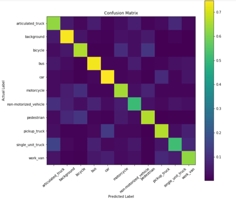
The confusion matrix demonstrates the accuracy and recall of the SVM validation on the training data. The y-axis represents the actual label of the training image, and the x-axis represents the label that we predict using our SVM. The values along the diagonal are probabilities, describing the chance for the SVM to correctly classify the image label.
Observing the results in the confusion matrix (Fig. 1), we can see that the SVM has difficulties identifying non-motorized vehicles, as it has the lowest recall value of correct identification, at 0.511. Also, it can be deduced that non-motorized vehicles are most often predicted as an articulated truck, when even to the human eye has very similar shape.
Confusion Matrix of KNN.
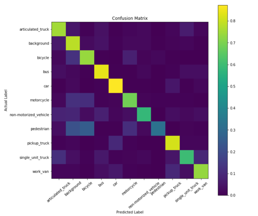
The confusion matrix of KNN shows us that it has trouble detecting pedestrians, as it classifies them as either background or bicycles. All three categories (bicycle, pedestrian, background) are categories that don’t show box shaped objects like cars, which would explain why they can be confusing to interpret. The general shape of a pedestrian is very similar to objects in a background (e.g. a pole); pedestrians can appear as a silhouette in background images. The shape of a human is also present in the bicycle images as a bicycle image intrinsically have a human in them.
To sum up our findings for the confusion matrices: the classes that are difficult for the SVM classifier are non-motorized vehicles and the classes that are difficult for the KNN classifier are pedestrians.
Moreover, to understand our cross-validation approach practically, we included a well-documented code along with this report.
In this part, we were asked to detect vehicles in several traffic images. Using a sliding window algorithm, HoG features were extracted from the traffic images and labeled via our classifiers from Part 2. The dataset for localization was different from the previous classification set. This dataset was called the MIO-TCD-Localization set. The localization dataset contained test and training images of 27,743 and 110,000 samples respectively. This gives a total of 137,743 samples in the localization set.
The approach taken to find a decent portion to train was implemented in two runs. The first run, we used the first 300 images of the entire training dataset because we assumed the data was randomized. The second run, we fetched the first 1000 images in the training set, then used the DICE coefficient to find the best 300 images. These are the images we decided to use, because we wanted to see what type of images best suit our localizer. The explanation and application for the DICE coefficient will be explained in Part 3.1.
In order to identify where a vehicle was, we ran a sliding window through the images. We built our sliding window using three passes, a squared, a vertical rectangle (2:3) and a horizontal rectangle (3:2) window. This was done because some of the images, (e.g. bicycles) have more of a vertical aspect to them, whereas others (e.g. bus, articulated truck) have more of a horizontal aspect to them. Our sliding window has 60% overlap, an area of 3600 pixels squared with a scale factor of 1.4. We chose 60% overlap because we wanted our window to be computationally fast while maintaining the image information as much as possible. We chose an area of 3600 pixels squared for the smallest window (starting) because the smallest images in our training set through our classifiers had features around that size. We chose a scale factor of 1.4 because we wanted our sliding window to stay within the image’s boundaries while scaling the sliding window as it gets closer to the camera of an image.
The theory behind implementing our sliding window was that when analyzing the vehicles, the ones that are located at the top of an image (further in the image) seemed smaller in pixel space compared to vehicles at the bottom (closer) of an image, which seemed bigger. As a result, we scaled our sliding windows to grow proportionally along the y-axis.
The localizer was based on the intersection between the SVM classifier and the KNN classifier. For a given sliding window, if both of the classifiers return the exact same label, then we can assume that an object was present, and we would save the position and dimension of this sliding window to compare with the ground truth bounding boxes. The reason why we chose to do this is because individually both classifiers had a lot of false positives. However, if we analyze them together we were able to filter out the false positives and keep most of the true positives. This will yield a better result. Additionally, we decided to reject all background and pedestrian images. We rejected background images since they are not vehicles and pedestrian images because they are too noisy. Also, since pedestrian images look similar to background images, it gave too many false positives, even when using both classifiers. Reflecting on our project, we would have trained our classifiers with more background and pedestrian images in order to differentiate both of them accurately.
Furthermore, the “motorized vehicle” label in the localization dataset represented vehicles too small to be classified in any of the other labels. As a result, we decided not to perform any pre-processing on the localization dataset. We assumed an object of this kind would be positively localized if it were labeled under one of the classification labels, with the exception of pedestrians and backgrounds since they are not vehicles. Different approaches could have been taken if we wanted to preprocess, such as parsing the ground truth csv file or deleting any bounding box associated with a “motorized vehicle” label. Subsequently, we decided not to discard the “motorized vehicle” label since we wanted to test the robustness of our localizer; which featured variable window sizes along the y-axis to account for small objects.
We evaluated our localizer by computing the DICE coefficient for the predicted vs. true bounding boxes. DICE coefficient is a measure of overlap between two images; a predicted bounding box and the ground truth bounding box. This measure ranges from 0 to 1, where 1 indicates perfect and complete overlap [5]. Equation (1) can be used to compute the DICE coefficient.

Equation (1) uses 3 parameters; True Positive (TP), False Negative (FN) and False Positive (FP). The True positive is the area where the predicted and the ground truth rectangles overlap. The False Negative is the portion of the ground truth rectangle that does not overlap with the predicted rectangle. The False Positive is the portion of the predicted rectangle that does not overlap with the ground truth rectangle.
The latter parameters had to be computed for every prediction and subsequently compared with the ground truth table provided with the dataset. A function was implemented in python to facilitate the computation of the DICE coefficient over the validation set. For a given image, this function computes the DICE coefficient for every possible combination of ground truth, predicted rectangles and determines the best match for each ground truth bounding box. A sequential approach was taken since a predicted rectangle can overlap multiple ground truth rectangles. In this case, for every ground truth rectangle, the best DICE coefficient needed to be determined while the others were discarded. This method prevents the distribution of the DICE coefficients over the whole dataset to be biased because of unrelated objects compared together. In other words, it maximizes the mean DICE by considering only the DICE coefficients of the matching bounding boxes for every image.
Additionally, in order to speed up our code, we vectorized our cross-validation function. Next, we compared a ground truth rectangle with a predicted rectangle. First, two NumPy arrays are initialized to 0 and to a shape equal to the shape of the test image. Second, the ground truth rectangle is drawn on one array and the predicted rectangle on the second array. The magnitude of the pixels inside the rectangle is set to 1.0 in order to perform Boolean operation arithmetically. Therefore, the two NumPy arrays can be seen as binary matrices, with each element representing a pixel on the test image. Third, the parameters of (1) are computed based on the two arrays. The overlapping section is obtained by multiplying (pixel-wise) the two arrays together. The result produces an array populated with 1’s where the rectangles overlap. This array is denoted as the overlapping array. TP is the sum of the overlapping array after it has been flattened. Finally, to get the other two parameters (FN and FP); FN is equal to the area of the ground truth rectangle’s area subtracted by the area of the TP, and FP is equal to the area of the predicted rectangle’s area subtracted by the area of the TP.
Moreover, the true bounding boxes were obtained from the csv file (gt_train) that was provided with the training images. This file contained labels and coordinates of all the predicted boxes for each image. For every predicted rectangle, we computed the DICE coefficient and compared it with all the possible combinations in the ground truth.
In order to evaluate our classifier, we used the localization predicted by our localizer. The following metrics were obtained: the accuracy, the prediction, and the recall of our localizer and classifier can be found on Table II.
Dice Coefficient Metrics
| Images | Dice Avg. | Standard dev. |
|---|---|---|
| Random 300 | 0.127 | 0.038 |
| Best 300 | 0.340 | 0.154 |
Mean DICE coefficient & standard deviation of localizer + classifier
The results in Table II are represented in the binomial distributions in Fig. 3 and Fig. 4.
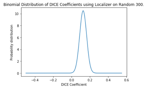
Binomial distribution of DICE coefficients of Random 300
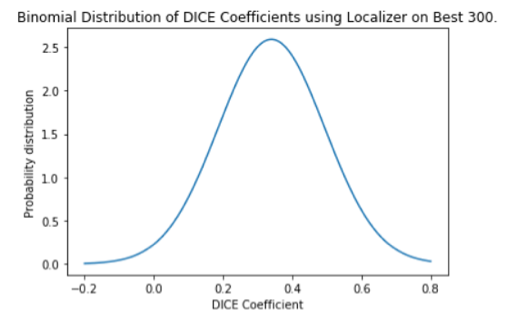
Binomial distribution of DICE coefficients of Best 300
Our localizer provides consistent results for the Random 300 run with the standard deviation being very low. Most of the DICE coefficient are located around the mean. On the contrary the Best 300 has a DICE coefficient that is farther apart, hinting to our hidden bias of choosing the best 300 images.
In order to evaluate our classifier, we used the localization predicted by our localizer. The following metrics were obtained: the accuracy, the prediction, and the recall of our localizer and classifier, which can be found on Table III.
Localization Metrics
| Images | Accuracy | Standard dev. | Precision | Recall |
|---|---|---|---|---|
| Random 300 | 0.460 | 0.042 | 0.112 | 0.338 |
| Best 300 | 0.586 | 0.055 | 0.297 | 0.645 |
Accuracy, prediction and recall of localizer + classifier
It can be noted that the values obtained in Table II describe a similar pattern for both the Random 300 and the Best 300 runs. The precision in both cases are low relative to the recall obtained. One reason to explain this is that our sliding window size was way too big compared to the ground truths. This would explain why FP is high (i.e. precision is low) compared to FN, which is low (i.e. recall is high). The accuracy of our localizer is also quite low for a localizer, signifying that not enough training images are used during the building of our classifier and/or not enough sliding windows are used per images in the localizer. Appendix III and Appendix IV show results of a sample result of the Random 300 and Best 300 runs respectively.
By comparing the results obtained in Table III with the ones obtained in Table I, we can see that there is a significant difference between the accuracy, prediction and recall. The parameters are much smaller when using the localizer instead of the classification data. One possible reason for this would be the challenge to deal with the variable size of the ground truth bounding boxes. The dimensions can vary significantly even for objects of the same class. Therefore, as mentioned earlier, the accuracy of our localizer is low. This is a reason why the classification using our localizer looks so bad compared to the classification using the classification data.
The values of recall and precision for Table I are almost similar, having a value of approximately 0.65 for SVM and 0.71 for KNN. Signifying that the amount of FPs and FNs is equal when performing classification using the classification data. However, the same observation cannot be made with the values of precision and recall in Table III, which are equal to 0.112 and 0.338 respectively for the random set of 300 images. This means that there are more FPs than there are FNs when performing classification using the localization data. To reiterate, a possible cause for this would be our window size, which is much larger than the ground truth bounding boxes. Another possible reason is our assumption of not having to pre-process the bounding boxes related to “motorized vehicle.” Certainly, it could have resulted in a lot of FPs since these objects are usually associated with very small bounding boxes compared to the size of our sliding windows.
Moreover, the background label of the classifier should not be included when evaluating the performance of the classifier. This is due to the fact that the purpose of training the classifier with background images is to be able to easily identify what is not part of the background, instead of trying to identify background scenes. Having a background label allows the classifier to be aware about the features of specific objects, which are usually not part of any other labels. For instance, if we train the classifier with images of bushes and trees, their features would probably be related to leaves and stems. These would be labeled in the background class, instead of being unknown and it would perhaps be associated with cars, motorcycles and so on. Thus, we don’t need to include the background labels because our goal is not to detect background.
The following project allowed us to dive into machine learning by understanding how to train a program using classification and localization algorithms. The initial part of this experiment was to train two classifiers, a support vector machine classifier (SVM) and K-Nearest-Neighbors (KNN) in order to classify given images of 11 categories. Finally, we implemented a localization method, that was based on the intersection between the SVM and the KNN classifier. We were able to classify the images and localize the objects using bounding boxes. Our code is also included with the report for reference. Possible improvements could be to use more images to train the classifiers or using the same number of images for every label except for the background label. Another improvement can be increasing the amount of background images used to build the classifier, this could positively affect the performance of our localization algorithm. It could decrease the amount of False Positives detected by introducing more features that are specific to background scenes. Additionally, using a more robust technique for the sliding window size could help substantially for localization. By assuming that the objects at the bottom of the images are bigger than the ones on top, we reduce the performance of the localization algorithm for some images, usually the ones with less depth (e.g. image 197 of localization training data). In some images, all the objects are on the same plane, meaning that a variable window along the y-axis is not necessarily suitable. Some techniques covered in class such as segmentation and GIST descriptors could be used for scene understanding. Such methods help understanding the direction of the depth and the relative distance of objects within an image. As a result, the sliding window size or the axis along which its size changes could be modified for each image based on the scene understanding and the direction of the motion.
Omitted from markdown.
Omitted from markdown.