For our final project we decided to extend our path tracer and turn it into a bidirectional path tracer. The way bidirectional path tracer works is by shooting rays from the eye (like in a forward path tracer) and from the light sources to form sub paths that are later combined to create full paths. Bidirectional path tracing takes advantage of Multiple Importance Sampling, a sampling method that weights different sampling techniques in order to choose the one that is most probable. As mentioned above, bidirectional path tracing works by shooting rays both from the eye and the light sources. We first create the eye sub paths the same way we do for a forward path tracer. We also build light sub paths that start from light and go in the opposite direction of the eye rays. When the pools of eye and light sub paths are created, we connect them by checking if there is an object in between both vertices. In out BPT, each vertex of a light sub path is connected to every vertex of an eye sub path. This way we achieve an extremely fast convergence in comparison with the forward path tracer. We allow diffuse and specular materials in our scene, as well as spherical light sources. We started our project by adding Multiple Importance Sampling to the forward path tracer. After MIS was implemented, we built the light sub paths. Finally, we connected the light and eye sub paths to create a bidirectional path tracer.
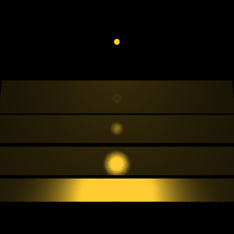
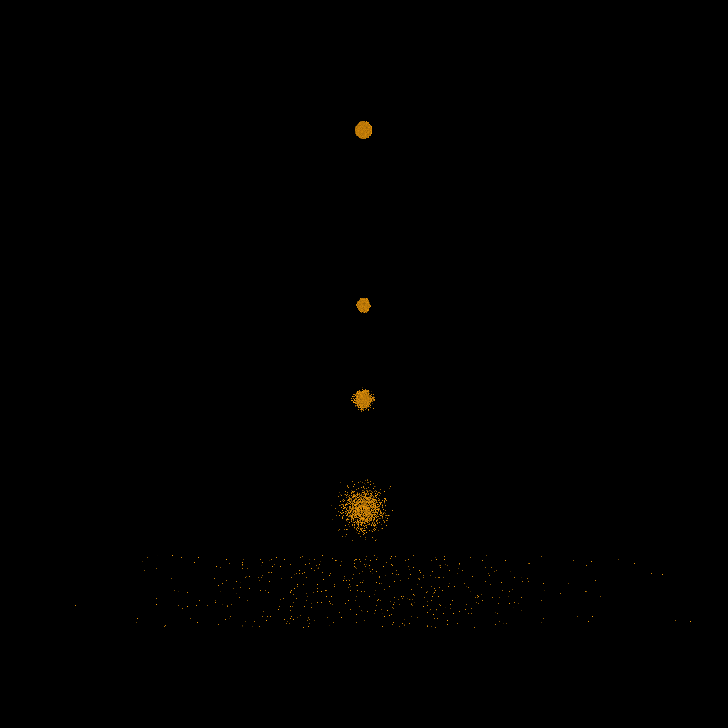
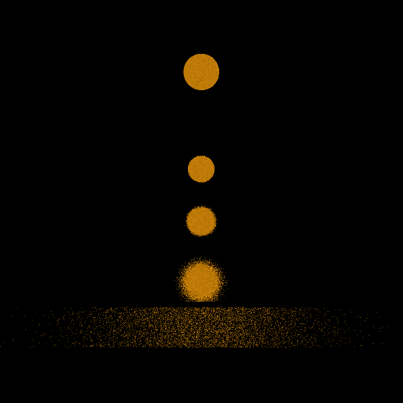
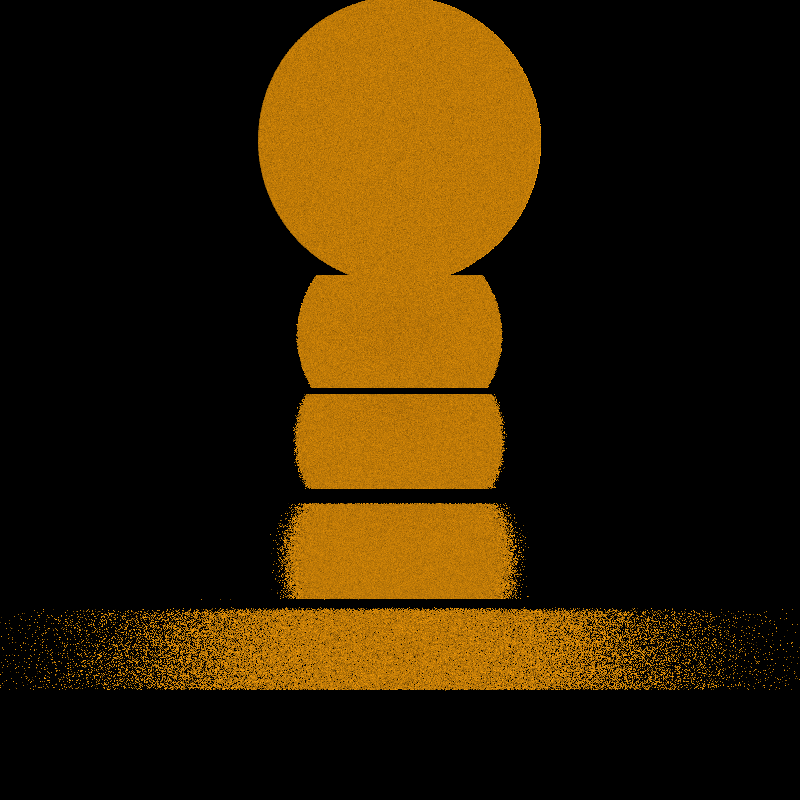
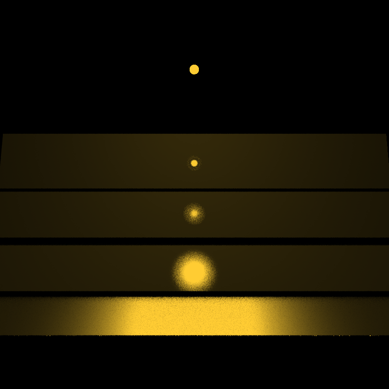
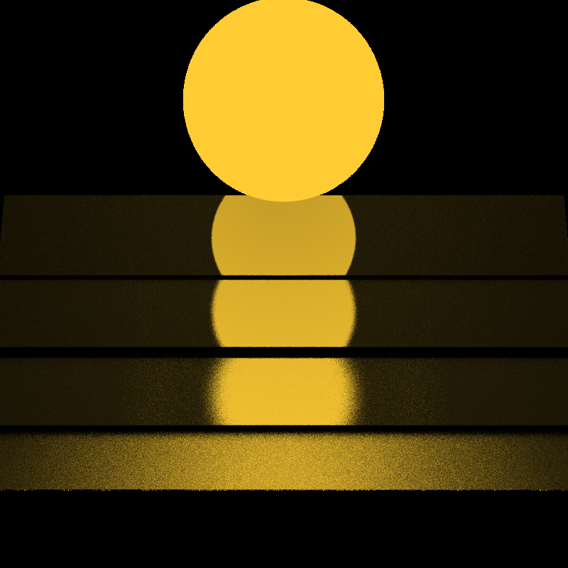
The way path tracing works is by shooting a ray from the camera into the scene and accumulate the colors at every hit point until a light source is reached. This method gives nice results for certain scenes, however it is not an efficient way for many other types of scenes (as we will show later.) Imagine you have a very small light positioned very far away from the scene. The probability of shooting a ray that is going to end up hitting that small light source is minimal. Here is where MIS comes into play. A more efficient way of calculating the final color of a pixel is by accumulating the color at every hit point but also shooting rays in the direction of the light source. That is sampling both the BSDF and the light. With MIS, we weight two different sampling methods using the balance heuristic and calculate the final color by weighting the contribution of both techniques. To test the effectivity of MIS we rendered three images containing fives shiny plates positioned at different angles and a light source that reflects on them. The planes range in specularity from most specular (back) to almost diffuse (front). The lights are all of the same power and color, but vary in size (radius of 0.2, 0.75, 2 and 3). The following images show the difference between sampling the BRDF and sampling the light sources.
 Veech Small DL
 Veech Small PT
 Veech med small DL
 Veech med small PT
 Veech med large DL
 Veech med large PT
 Veech large DL
 Veech large PT
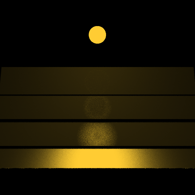
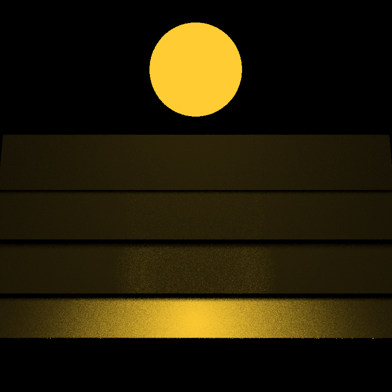
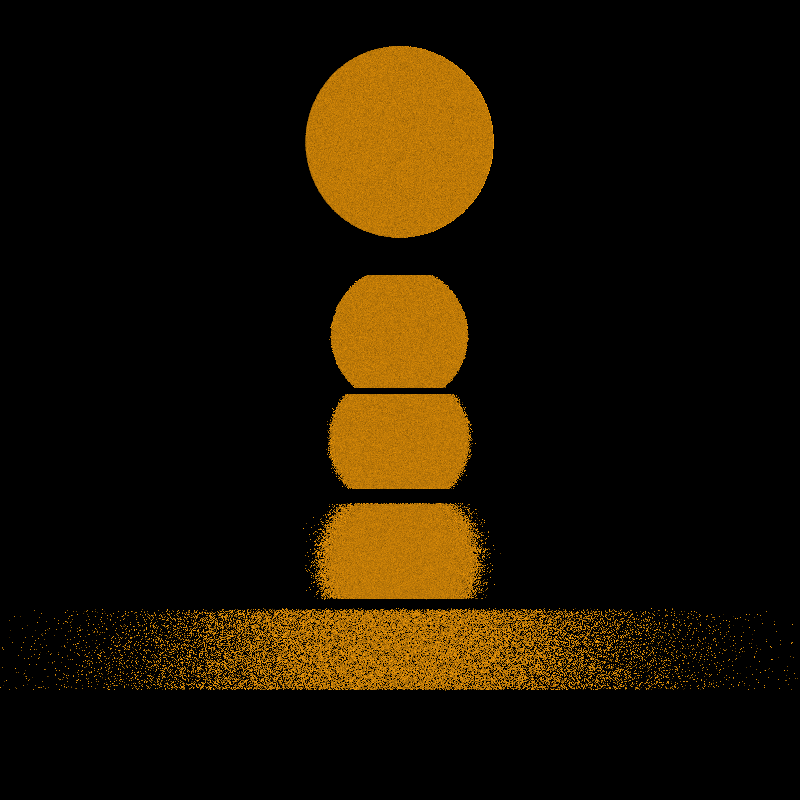
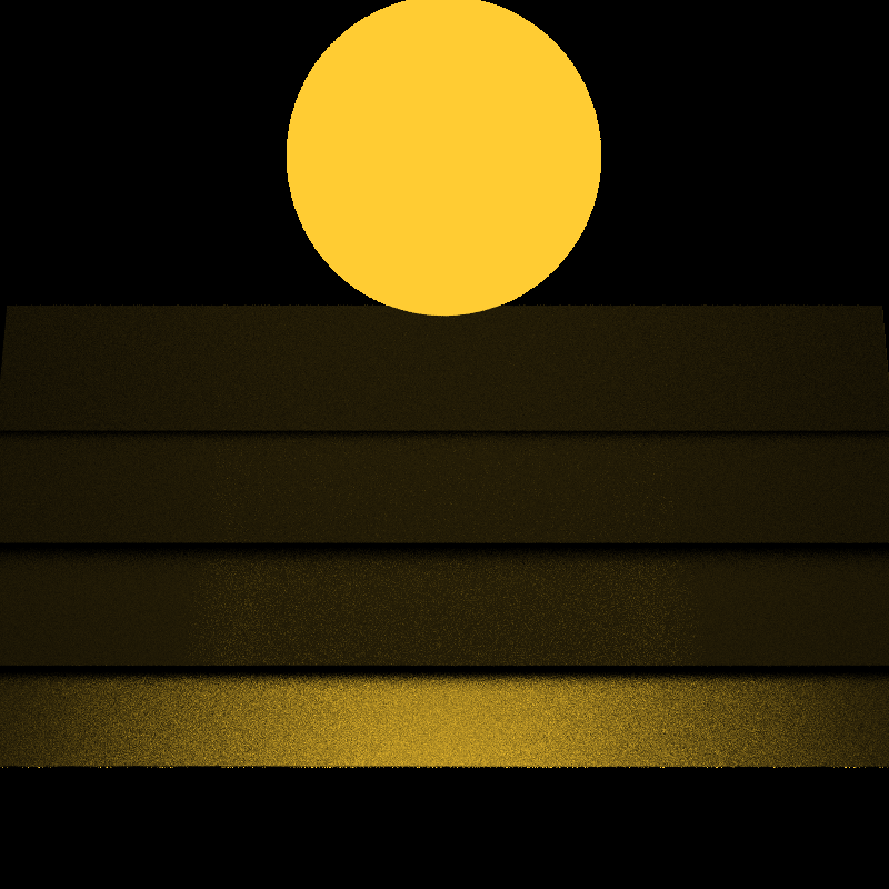
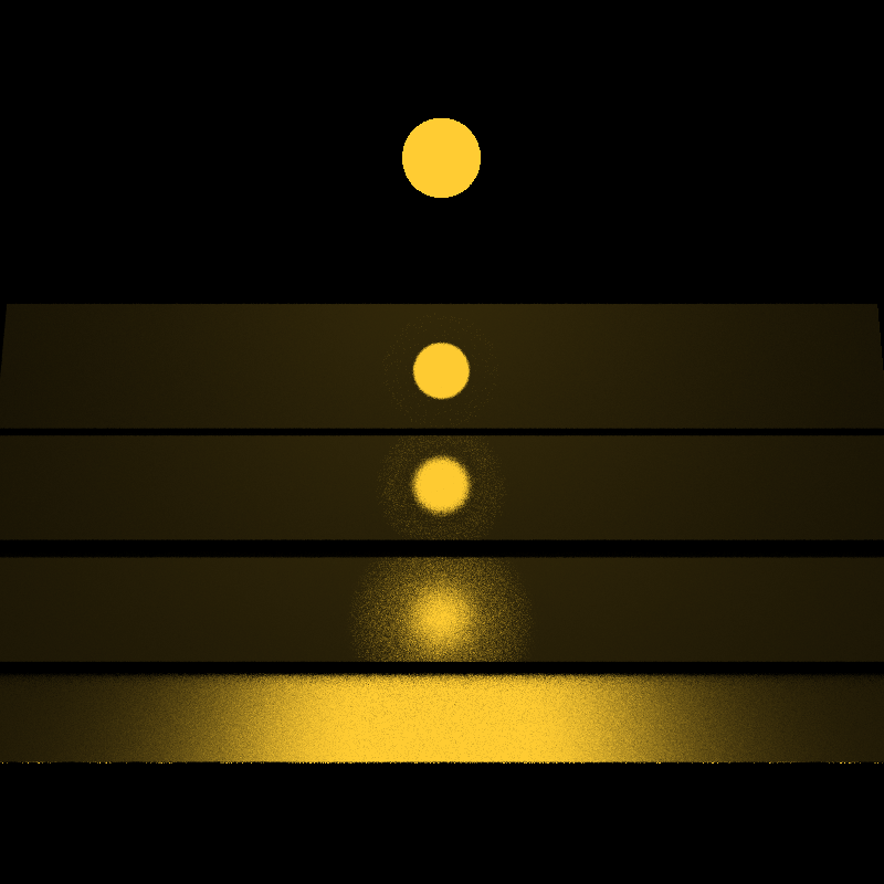
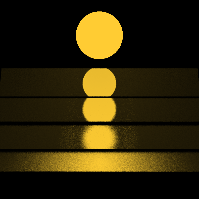
These sampling techniques differ on the variance, depending on the radius of the light source and the shininess of the plate. For example, as the images show, for small light and almost diffuse plate, sampling the light source gives a better result than sampling the BSDF. The opposite occurs for big light sources and shiny materials. The following images show the same test, however now instead of sampling one of each technique, we combine them and weight them to decrease the variance of the previous sampling methods. With MIS we choose which technique is better in each case, and weight this “right” technique more to achieve a more accurate result.
 bidirectional small
 bidirectional med small
 bidirectional med large
 bidirectional large
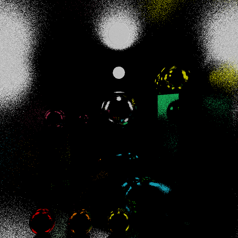
To show the robustness of our implementation we render a complex scene of 14 specular objects with 2, 10, 100 and 1000 iterations. The following image (only 2 iterations) shows the fast convergence of our implementation.
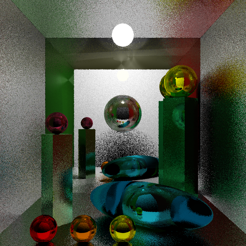 BPT Performance 2 iters
The next picture (1000 iterations) was rendered to compare final times with forward path tracer, but this render was unnecessary for other purposes, since the image converges at around 100-200 iterations. We choose a trace depth of 4, and it is clearly shown in the pictures that forward path tracing is not able to render such scene in less than 1000 iterations. Even though the time per iteration is faster for forward path tracing (126.283 vs. 460.105) it is clear that BPT converges faster.
BPT Performance 1000 iters
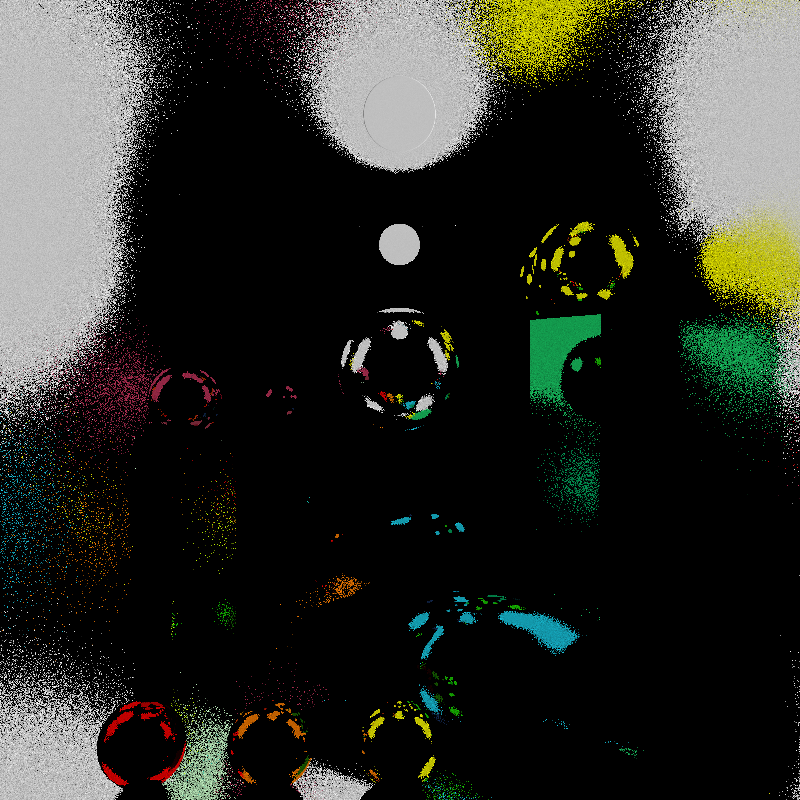 FPT Performance 1000 iters
Here is the same comparison with 100 iterations.
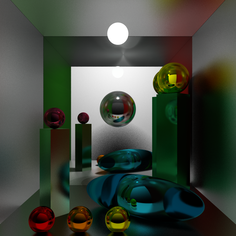 BPT Performance 100 iters
 FPT Performance 100 iters
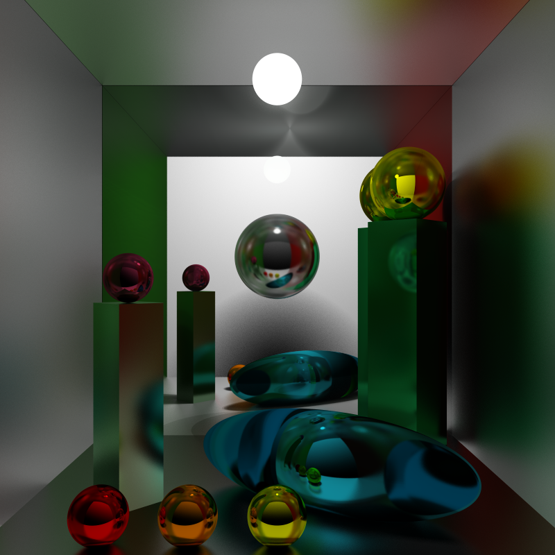
Here is another scene we rendered. This time we included Depth of Field as well, which is virtually free for both the Forward and Bidirectional PathTracer.
This scene has
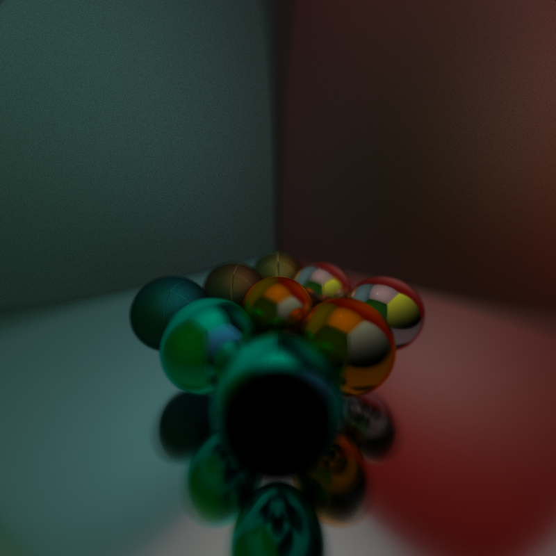
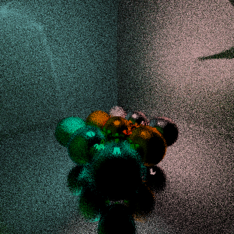 The Forward path tracer was allowed to run for 3000 iterations which took approximately 16 minutes. Which comes out to approximately .33 seconds/iteration.
The Bidirectional Path tracer was allowed to run for 500 iterations which took approximately 18 minutes. This is approximately 2.15 seconds per iteration. As we will see below, each iteration takes significantly more time than in the standard pathTracer, however with small lights it produces a much more pleasing image in the same amount of time.
The Forward path tracer was allowed to run for 3000 iterations which took approximately 16 minutes. Which comes out to approximately .33 seconds/iteration.
The Bidirectional Path tracer was allowed to run for 500 iterations which took approximately 18 minutes. This is approximately 2.15 seconds per iteration. As we will see below, each iteration takes significantly more time than in the standard pathTracer, however with small lights it produces a much more pleasing image in the same amount of time.
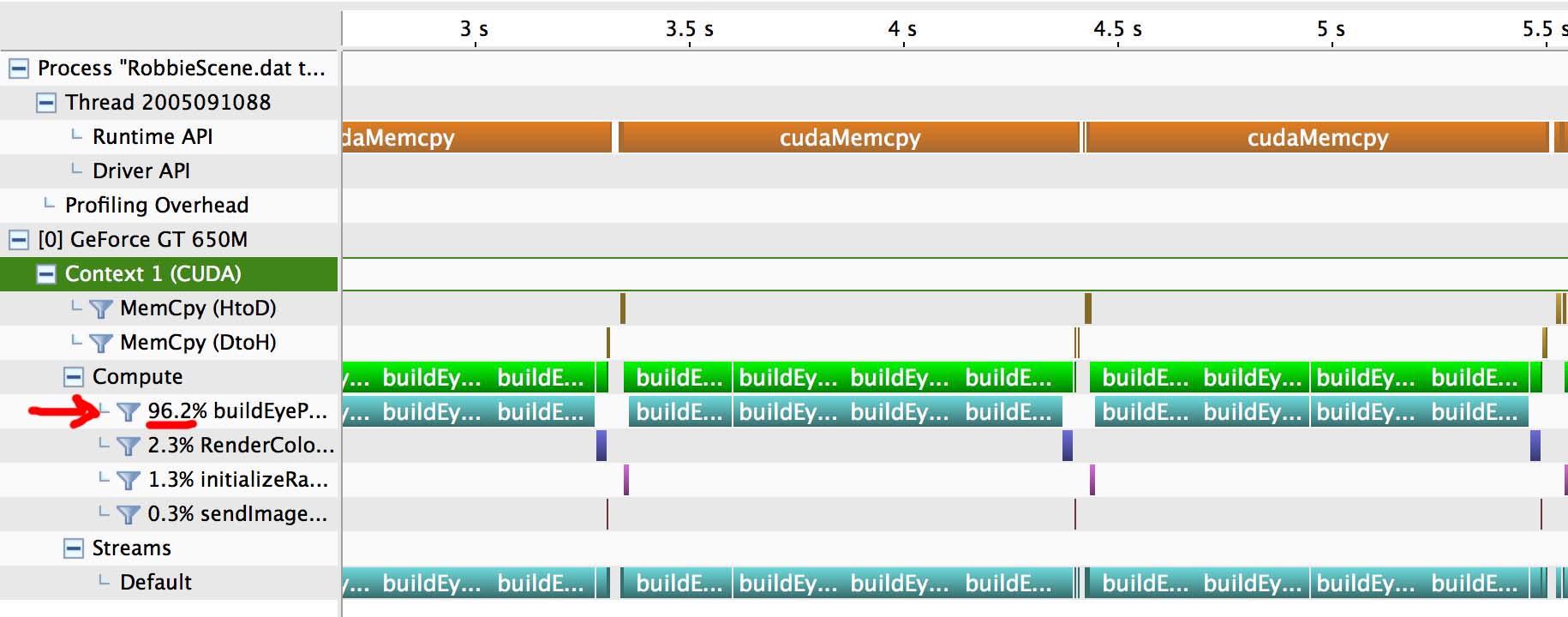
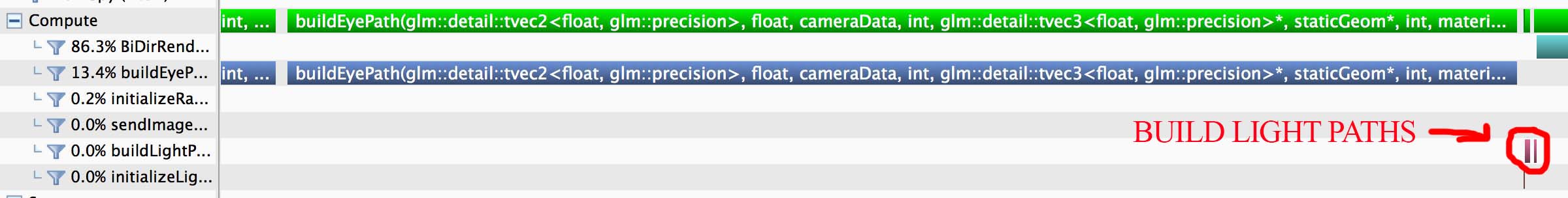
We ran the profiler for both the forward path tracer and the bidirectional path tracer. The folowing data was gathered when running the scene above with the Depth of Field and the 9 spheres. The scene consists of 15 objects, there were 12 specular surfaces, 2 diffuse, and one light.
For forward path tracer we observe that 96% of the work was spend in the buildEyePath kernel, which crate the pool of rays from the camera into the scene. This is where all of the object intersections occur.
For bidirectional path tracer, however, the most expensive kernel is the BiDirRenderColor, which connect the light and eye sub paths. The reason for this is we have to test intersections between each light subpath vertex and each eye path vertex. This means that the kernel does n^2 intersection tests instead of n where n is the trace depth.
In addition, in our implementation we actually connected 5 light paths to each eye path instead of just one. This meant there were 5n^2 intersection tests instead of n. Therefore the connection kernel easily dominates the running time.
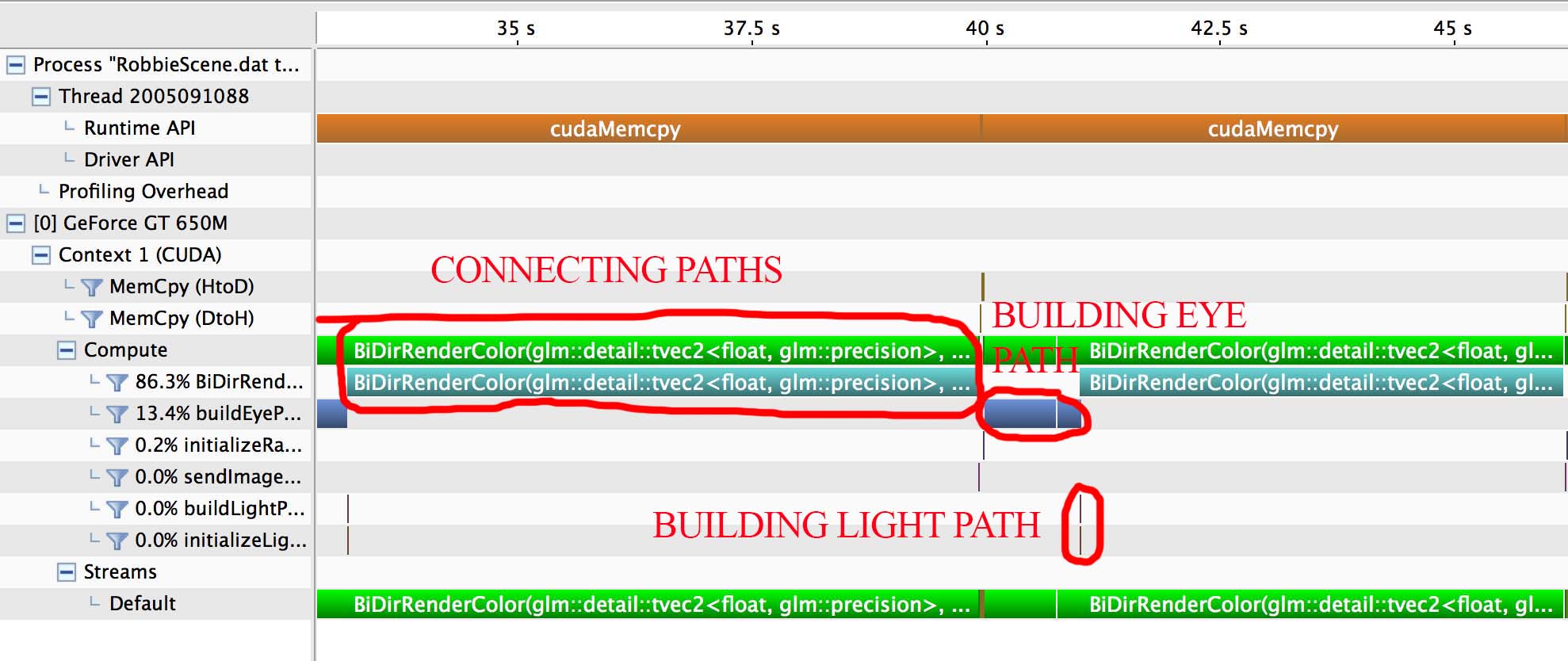
In the Bidirectional Pathtracer, 13.4% is spend in the eyePathKernel. LightPathKernel, which build the light paths is not as expensive as building the eye paths. This is because our pool of rays is of size (numberOfPixels) which for us was 160,000 while for light paths we only generated 10 each iteration.
 It is worth noting that we have not included any acceleration structures in our pathtracer and we have run with a small number of objects. If we were to render a scene with much complexity at all we would benefit greatly from bounding boxes and other structures that can reduce our number of intersection tests.
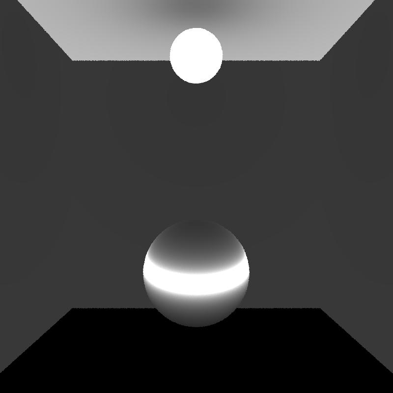
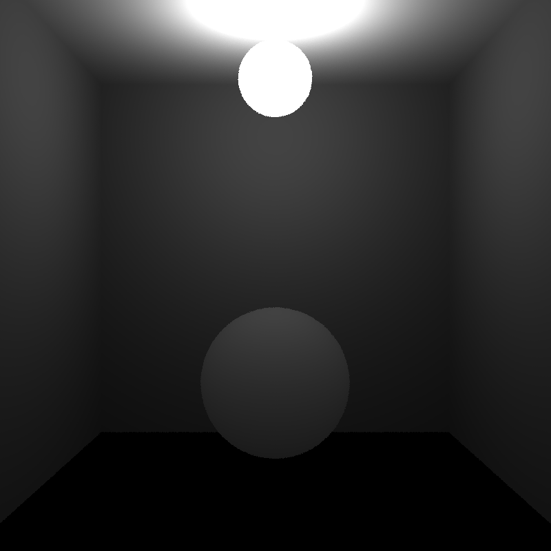
During the process we noticed we were getting some strange artifacts in our image. This debug view renders the solid Angle calculated at each position. Notice the band on the sphere and the ceiling in the incorrect image as compared to the correct one. This helped us find a wildly incorrect transformation in our implementation.
 BAD Solid Angle
 good Solid Angle
- Robust Monte Carlo Methods for Light Transport Simulation – Eric Veach
- Bi-directional Path Tracing – Eric P. Lafortune and Yves D. Willems