REANA example - LHCb Rare Charm Decay Search

About

This analysis example attempts to reproduce LHCb rare charm decay study published in Phys. Lett. B 724 (2013) 203-212.

These decays are very rare, which makes their observation extremely challenging. The LHC produces a lot of charm particles $D$, but it also produces a much greater number of other particles which can be mistaken for the signal. It is necessary to develop an effective strategy to identify the signal events in the large data sample. The event selection strategy is implemented in three stages: the trigger selection, stripping selection and the multivariate analysis.

In the paper, you can lean more about the theoretical background and motivation to study this decay.

This example is based on this analysis-case-study.

Analysis structure

Making a research data analysis reproducible basically means to provide "runnable recipes" addressing (1) where is the input data, (2) what software was used to analyse the data, (3) which computing environments were used to run the software and (4) which computational workflow steps were taken to run the analysis. This will permit to instantiate the analysis on the computational cloud and run the analysis to obtain (5) output results.

1. Input data

The data being used is currently only available on request. It consists of a 10 GB ROOT file.

2. Analysis code

You can straightforwardly run the analysis step by step as explained below:

$ mkdir -p results/tmp && mkdir -p logs
$ root -b -q 'Optimise.C("${data}", "results")' | tee logs/optimise.log
$ root -b -q 'ModelFixing.C("${data}", "results/tmp/PhiModels.root")' | tee logs/model_fixing.log
$ root -b -q 'OSMassFit.C("${data}", "results/tmp/PhiModels.root", "results")'  | tee logs/massfit.log

Headers and Plot style:

• lhcbStyle.C - Plot formats specific to the LHCb collaboration.

• RooFitHeaders.h - Libraries and packages needed to perform the fitting.

Step 1: Optimisation stage Optimise.C

Optimisation is the process where combinations of different variable cuts are evaluated in order to maximise the signal yield and reduce the background. In this analysis, the optimisation study is performed to choose the combined BDT and particle identification (PID) selection criteria that maximise the expected statistical significance. The result of the script is the heat map called 2D_Optimisation_Pi.pdf. The higher significance (in yellow) means cleaner signal. The optimal significance is found to be at the cuts of BDT > 0.1 and PIDmu > 2.

$ root -b -q Optimisation.C(<data_file>, <results_directory>)

Step 2: Theoretical Model Fixing stage ModelFixing.C

Creates the theoretical model that the fit is compared to.

$ root -b -q ModelFixing.C(<data_file>, <tmp_phi_models>)

Step 3: Mass Fitting stage OSMassFit.C

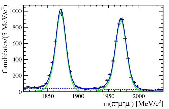
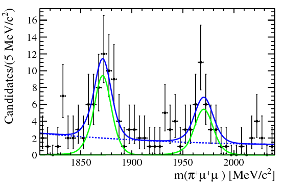
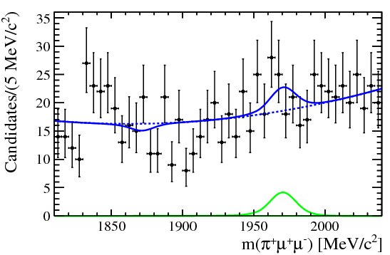
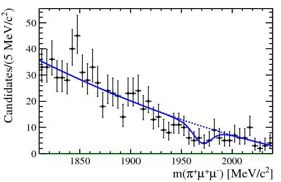
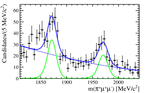
The fit for the signal was modelled with the sum of Crystal Ball distributions. Each shape consists of a Gaussian core with a power law tail on opposite sides. The background was modelled with a 2nd order Chebyshev polynomial distribution.

$ root -b -q OSMassFit.C(<data_file>, <tmp_phi_models>,  <results_directory>)

3. Compute environment

In order to be able to rerun the analysis even several years in the future, we need to "encapsulate the current compute environment", for example to freeze the ROOT version our analysis is using. We shall achieve this by preparing a Docker container image for our analysis steps.

Some of the analysis steps will run in a pure ROOT analysis environment. We can use an already existing container image, for example reana-env-root6, for these steps.

4. Analysis workflow

This analysis example consists of a simple workflow the theoretical model is generated and used for fitting.

The analysis workflow consists of the above mentioned stages:

              START
               |
               | D2PiMuMuOS.root
               |
               V
+------------------------------+
| (1) Optimisation             |
|                              |
|    $ root Optimise.C ...     |
+------------------------------+
               |
               | 2D_Optimisation_Pi.pdf
               | MuMuMass_Pi.pdf
               | PhiModels.root
               |
               V
+------------------------------+
| (2) Theoretical Model Fixing |
|                              |
|    $ root ModelFixing.C ...  |
+------------------------------+
               |
               | PhiModels.root
               V
+------------------------------+
| (3) Mass Fitting             |
|                              |
|    $ root OSMassFit.C ...    |
+------------------------------+
               |
               | low_dimuon_signal.pdf
               | high_dimuon_signal.pdf
               | eta.pdf
               | rho_omega.pdf
               | phi.pdf
               |
               V
              STOP

For example:

$ root -b -q 'Optimise.C("data.root", "results_directory")'
$ root -b -q 'ModelFixing.C("data.root", "phimodels.root")'
$ root -b -q 'fitdata.C("data.root", "phimodels.root", "results_directory")'

Note that you can also use CWL or Yadage workflow specifications:

• workflow definition using CWL
• workflow definition using Yadage

5. Output results - Mass fit

The result of this analysis are the following plots in various dimuon mass ranges. We studied the three body decay in high dimuon and low dimuon mass range, and we did not observe any signal.

Dimuon resonances	Dimuon mass range (MeV)	Plot
Three body decay (low dimuon)	250 - 525	low_dimuon_signal.pdf
$\eta$	525 - 565	eta.pdf
$\rho , \omega$	565 - 850	rho_omega.pdf
$\phi$	850 - 1250	phi.pdf
Three body (high dimuon)	1250 - 2000	high_dimuon_signal.pdf

The plots can be found in the mass_fits folder at the end of the execution.

One of the final plots, representing the $\phi$ contribution, is shown below.

Running the example on REANA cloud

We start by creating a reana.yaml file describing the above analysis structure with its inputs, code, runtime environment, computational workflow steps and expected outputs:

version: 0.6.0
inputs:
  files:
    - Optimise.C
    - ModelFixing.C
    - OSMassFit.C
    - RooFitHeaders.h
    - lhcbStyle.C
    - data/D2PiMuMuOS.root
  parameters:
    data: data/D2PiMuMuOS.root
workflow:
  type: serial
  specification:
    steps:
      - environment: 'docker.io/reanahub/reana-env-root6'
        commands:
        - mkdir -p results/tmp && mkdir -p logs
        - root -b -q 'Optimise.C("${data}", "results")' | tee logs/optimise.log
        - root -b -q 'ModelFixing.C("${data}", "results/tmp/PhiModels.root")' | tee logs/model_fixing.log
        - root -b -q 'OSMassFit.C("${data}", "results/tmp/PhiModels.root", "results")'  | tee logs/massfit.log
outputs:
  files:
    - results/2D_Optimisation_Pi.pdf
    - results/MuMuMass_Pi.pdf
    - results/low_dimuon_signal.pdf
    - results/high_dimuon_signal.pdf
    - results/eta.pdf
    - results/rho_omega.pdf
    - results/phi.pdf

We can now install the REANA command-line client, run the analysis and download the resulting plots:

$ # create new virtual environment
$ virtualenv ~/.virtualenvs/myreana
$ source ~/.virtualenvs/myreana/bin/activate
$ # install REANA client
$ pip install reana-client reana-cluster
$ # connect to some REANA cloud instance
$ export REANA_SERVER_URL=https://reana.cern.ch/
$ export REANA_ACCESS_TOKEN=XXXXXXX
$ # create new workflow
$ reana-client create -n my-analysis
$ export REANA_WORKON=my-analysis
$ # upload input code and data to the workspace
$ reana-client upload ./*.C ./*.h ./data
$ # start computational workflow
$ reana-client start
$ # ... should be finished in about 15 minutes
$ reana-client status
$ # list output files
$ reana-client ls | grep ".pdf"
$ # download generated plots
$ reana-client download

Please see the REANA-Client documentation for more detailed explanation of typical reana-client usage scenarios.