Framework for modeling, detecting and visualizing objects through superquadric functions.
superquadric-lib.
- Theoretical background
- Dependencies & how to compile
- Module structure
- Use case & results
- Documentaion & more
The superquadric-model framework is based on the idea that low-dimensional, compact, mathematical representation of objects can provide computational and theoretical advantages in hard problems trackled in robotics, such as trajectory planning for exploration, grasping and approaching towards objects. It takes inspiration from theories conceived during the 90's and 2000's (Jaklic, A., Leonardis, A., Solina, F., Segmentation and Recovery of Superquadrics, Ch. no. 2, Springer, 2000 (1)) since it uses superquadric functions as a mathematical and low dimensional model for representing objects. The novelty of the superquadric-model module consists in the implemention of the standard optimization problem provided by (1) by exploiting the Ipopt software pacakge (for software documentation: Ipopt, for theroetical background: A. Watcher, L.T.Biegler, On the Implementation of an Interior-Point Filter Line-Search Algorithm for Large-Scale Nonlinear Programming, 2004 (2)). Furthermore, the reconstructed superquadric is overlapped in real-time on the real scene seen by the robot's cameras.
The so called inside-outside superquadric function is given by:
and it provides a simple test whether a given point lies inside or outside the superquadric. If F < 1, the given point ( x, y, z) is inside the superquadric, if F = 1 the corresponding point lies on the surface of the superquadric, and if F > 1 the point lies outside the superquadric.
The inside-outside function can be used for superquadric recovery. Suppose we have a set of 3D surface points, for example coming from a stereo video system, ( xi, yi, zi ), i = 1, .., n. The superquadric in general position is defined by the following equation:
We want to find such values for the 11 parameters Λ ( λj, j = 1, .. 11 ) that most of the n 3D points will lay on, or close to the superquadric surface. The superquadric parameters have the following meanings:
- λ1, λ2, and λ3 are the semi-axes lengths;
- λ4 and λ5 are the exponents, responsible for the superquadric shape;
- λ6, λ7, and λ8 are the coordinates of the superquadric center;
- λ9, λ10, and λ11 are the Euler angles, representing the superquadric pose.
The problem can be solved by minimizing the following quantity:
The F function is raised to the power of ε1 in order to make the error metric independent from the shape of the superquadric and provide faster convergence. This change causes a bias towards larger superquadrics. This effect is compensated by the multiplication with the term λ1, λ2, λ3 which is proportional to the volume of the superquadric.
More information are available in our ICRA paper [1].
In Linux systems code can be compiled as follows:
git clone https://github.com/robotology/superquadric-model.git
cd superquadric-model
mkdir build; cd build
ccmake ..
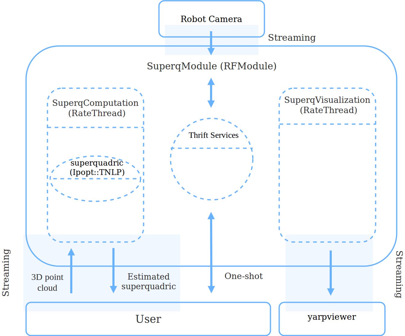
make installThe module structure is outlined in the following picture:
The superquadric-model module launches two separate threads:
SuperqComputation, computing the superquadric given the 3D point cloud of the object;SuperqVisualization, showing the estimated superquadric or the points used for the computation (optional).
The superquadric-model also provides some thrift services through a rpc port. The user can communicate with the module through these services in order to ask the state of the two threads or to modify some parameters on the fly.
The module also receive the camera image and, if the SuperqVisualization is enabled, the output is shown on a yarpview.
The SuperqComputation provides two buffered ports, respectively for receiving continuosly the 3D point cloud of the object and for sending the estimated superquadric. The computation and visualization threads also share some variables, such as the computed superquadric.
In order to improve the superquadric modeling, the SuperqComputation thread provides two filtering process:
- on the 3D point cloud;
- on the estimated superquadric.
The former is a density filter, discarding noisy queues of the point cloud, that can arise from the noise of the disparity map.
The latter is a median filter with an adaptive moving window. Each filtered superquadric is obtained by applying a median filter on the last m estimated superquadrics. The value of m depends on the estimated velocity of the object. If the object is moving the window width is low in order to correctly track the object (e.g. _m_=1), otherwise m is incrementally increased up to a maximum value.
The superquadric-model module requires the 3D point cloud of the object we want to model with a superquadric function.
An example code for retriving this information, together with a tutorial, is provided in the folder tutorial in this repository.
Here is an example of a reconstructed superquadric:
The execution times are respectively:
- for superquadric computation nearly 0.1 s (including the median filter on the estimated superquadrics)
- for point cloud filtereing nearly 0.1 s (optional)
- for visualization nearly 0.01 s (optional)
This video shows the superquadric modeling of several objects.
You can find an overview of the entire pipeline superquadric-model module + example code in the following pdf: superquadric-model.pdf.
If you want to browse the prezi version of the presentation, you can have a look at the link: superquadric-model-prezi.
Online documentation is available here: http://robotology.github.com/superquadric-model.
Material included here is Copyright of iCub Facility - Istituto Italiano di Tecnologia and is released under the terms of the GPL v2.0 or later. See the file LICENSE for details.
[1] G. Vezzani, U. Pattacini and L. Natale, "A grasping approach based on superquadric models", IEEE-RAS International Conference on Robotics and Automation 2017, pp 1579-1586.


