-
Notifications
You must be signed in to change notification settings - Fork 10
Understanding Read Correction
In an ideal world, a genetic sequencer would detect every base in each chromosome with complete certainty. It would start at the telomere of each p-arm, proceed through the centromere, and end at the tip of the q-arm. It would do this once for each chromatid, and output a FASTA file containing each base present. Variant calling would be a simple matter of comparing each base to a genetic reference, and structural variant detection would be trivial.
In the real world, all instruments introduce a non-zero amount of random error. Modern short read sequencers produce results with impressive accuracy, but still include a small but unavoidable amount of systematic and random error. These errors can be detected and corrected by taking advantage of oversampling and statistical analysis.
The process of examining the body of read data and correcting (or removing) erroneous bases is called Read Correction. It is particularly critical for creating graph structures of read data, because erroneous bases lead to complicated graph structures.
Consider a 50X WGS in FASTQ format. At 150 bases per read, the dataset will contain roughly 1 billion reads. With an error rate of 0.1%, we should expect an average of at least 1 error in 1 million reads, or roughly 150 million total erroneous bases. In a graph structure, each of these errors represents a path deviation that must be represented and considered for analysis. Since these errors are largely unique, this can significantly impact performance, wasting time and memory on paths with no real evidence to support them.
BioGraph uses a Read Correction method that is highly efficient and eliminates errors with virtually no impact on the ultimate set of variant calls. It works without the need to consider quality scores, and thus requires no base quality score recalibration step. The process is completely reference-free, eliminating the possibility of reference bias.
Read errors are corrected using a novel implementation of the A-star (A*) path-finding algorithm to find globally optimal base substitutions. This step is divided into two parts: k-merizing the reads and then using "good" kmers to infer the base substitutions needed to correct the reads.
K-mers are generated from the reads during the import process. The default k-mer size is 30. Below is an example given a k-mer size of 6:
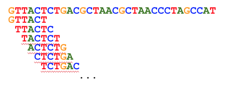
All kmers from all reads are counted using a high-performance multi-pass bloom filter:
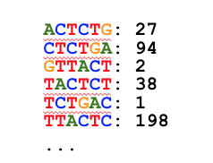
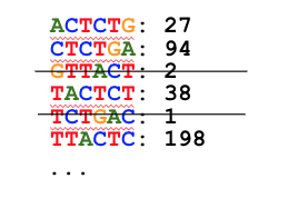
K-mers less abundant than a threshold (default: 4 or less) are discarded:
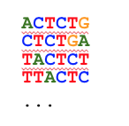
The remaining k-mers are considered “true”. The counts are discarded:
The k-mers are then counted, and a distribution of k-mer counts is considered.
If we plot the k-mer counts for a 30X WGS on a graph, we see a bimodal distribution:
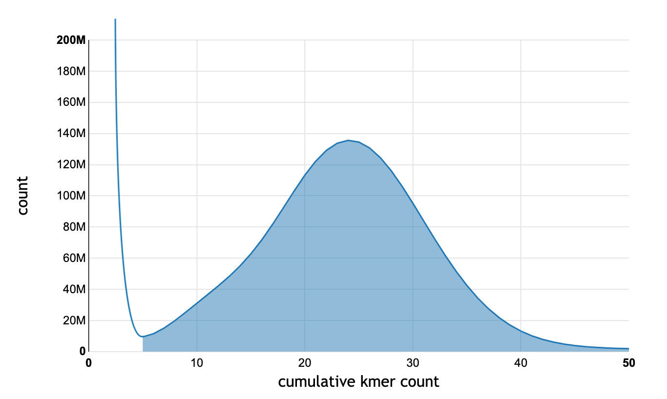
A typical k-mer count distribution. The k-mers to the right of the cutoff (count ≥ 5) are shaded blue, and are used for read correction. The k-mers to the left of the cutoff (< 5) are discarded.
A cutoff is chosen near the minimum point between the two peaks. Any k-mers to the left of the cutoff are considered erroneous and are removed. The remaining kmers are then used to correct the reads.
A de Bruijn graph is constructed from the remaining set of true k-mers, as if for de novo assembly. This graph represents an error-free reconstruction of the true read sequences. It allows for computationally efficient identification of error-free reads and correction of erroneous bases in all other reads using the A* search algorithm.
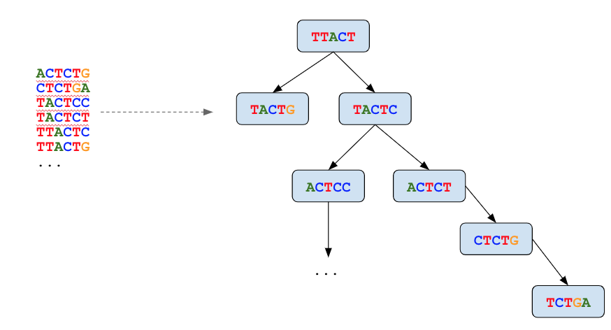
Reads where all k-mers map perfectly to the graph do not require correction.

For reads that imperfectly map to the graph, one or more globally optimum base substitutions are located so that the read aligns to the graph with no mismatches and differs by the smallest possible number of changes from the original read.

Read errors often occur at the end of the read. Bases may be automatically trimmed during read correction. Correction starts at the beginning of a read up to the maximum allowed number of base substitutions (by default 8). Once this number of bases substitutions is reached, the read is trimmed starting from the next erroneous base. An example using a default of a maximum of 3 corrections follows:

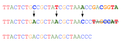
The total number of bases corrected and the fraction of reads that may be automatically trimmed can be selected as appropriate for your dataset. By default, up to eight bases may be corrected (requiring a minimum of two good bases between them), and reads may be trimmed automatically down to a minimum of 70% of the original length. Reads that cannot meet the read correction criteria are discarded.

Processing then proceeds with the resulting error-corrected reads.
We benchmarked the read correction step using data simulated with Mason (http://www.seqan.de/apps/mason/). We simulated reads for whole human genome sequencing experiments on human reference hg19 using an Illumina HiSeq machine with 30x, 45x and 60x coverage.
| Read depth | Total read count | Reads w/o errors before correction | Remaining after correction | Reads w/errors before correction | Error reads corrected |
|---|---|---|---|---|---|
| 30x WGS | 32166263 | 20522011 | 20521863 | 11644252 | 10579162 |
| 45x wGS | 48252264 | 30785990 | 30785933 | 17466274 | 15957764 |
| 60x WGS | 64330880 | 41034875 | 41034827 | 23296005 | 21388977 |
Approximately 91% of reads with an error are corrected. The remaining approximately 9% of reads with errors are discarded. This makes up approximately 3% of the total number of reads.