I made an internship at the Universidad Carlos III de Madrid of one month. This internship was done as part of my electrical engineering degree. I completed my intership in the Department of Computer Science and Engineering laboratory. I want to thank Miguel Angel Patricio to introduce me in this internship and Juan Pedro Llerena Cana to have taken the time to explain me things about my project.
In the immediate context of smart cities in which use drones is multidisciplinary, it is essential that they be able to carry out missions independently. To carry out these missions it is necessary that drones be able solve problems associated with obstacles detection.
Currently, many sensors are used for this purpose, but given the limiting factor of weight and the increase in computing capacity of current systems, use cameras is of great interest.
In this project, the using of camera embeds computer vision to extract interesting informations (obstacles in our case). Computer vision is an interdisciplinary scientific field that deals with how computers can be made to gain high-level understanding from images or videos. More specifically, computer vision is the construction of explicit and clear descriptions of objects in an image. It involves the development of a theoretical and algorithmic basis to achieve automatic visual understanding. Computer vision tasks include methods for acquiring, processing, analysing and understanding digital images.
Computational-based navigation of autonomous mobile robots has been the subject of more than three decades of research and it has been intensively studied. Processing images in real time is critical for decision making during the flight.
In the context of autonomous drones, the aim of the project is to detect all the objects surrounding the device during his flight. In computer vision, an element detected and recognized by the system is named class (or label). Class can be anything like people, car, road, window, tree ... Therefore, in this project, we have to detect lot of classes in real-time to change the drone direction if he spots an obstacle (class for the robot). To recognize classes, one model has been trained thanks to a machine learning process. A machine learning model can be a mathematical representation of a real-world process. To generate a machine learning model, it is necessary to provide training data to a machine learning algorithm to learn from. We can understand the whole computer vision in this scheme :

Recent developments in neural networks have greatly advanced the performance of visual recognition systems. Visual recognition tasks such as image classification, localization and detection are key components of computer vision. In this report, we are going to present several neural networks architectures which helped me to progress in my project.
To bring a computer vision system on a drone, we have to install system small and robust. A cheap idea is the utilisation of Raspberry Pi due to its size and its I/O on board which enables to integrate a camera and a SD card effortless. Rasbperry Pi uses operating system such as Raspbian, a Debian-based distribution, so we are able to install Python and other packages to developp our computer vision applications. But, to be realistic, a Raspberry Pi as fast alternative is unable to match the modern PCs.
In order for the drone to support a computer vision system, we will use a Raspberry Pi for this project. To code computer vision systems, we are going to use in particular a famous library of Python : OpenCV. OpenCV supports a lot of algorithms related to Computer Vision and Machine Learning and it is expanding day-by-day.
To start my project, the first thing I had to do was setup Rasbpian on my Raspberry. I choose to download the Raspbian Buster with desktop version because I thought I might need a screen to see what the camera is displaying. Therefore, I have downloaded this version and I have wrote the Raspbian disc image to my SD card thanks to Balena Etcher.
https://thepi.io/how-to-install-raspbian-on-the-raspberry-pi/
Once it was done, I installed Python 3 and OpenCV on the Raspberry Pi.
After this, I configure my Python virtual environment to develop correctly. A virtual environment is a Python tool for dependency management and project isolation. This allows Python libraries to be installed locally in an isolated directory for a particular project, as opposed to being installed globally.
To create a virtual environment for a project we’re working on called test-project, you have to go in this folder and create the virtual environment.
python3 -m venv venv_name/
The only thing left to do is to “activate” our environment by running the scripts we mentioned. Do not forget to do this when you want to work on the test-project.
source venv/bin/activate
When we’re done working on our project, we can exit the environment with
deactivate
SSH (also known as ‘Secure Shell’) is an encrypted networking technology that enables you to manage computers from the command line over a network. SSH is the best method of connecting to your Raspberry Pi.
Two conditions are necessary for the connection : your computer has to be on the same network of the Raspberry Pi and the SSH has to be enable on the Rasbperry Pi.
To connect you remotly on the Rasbperry Pi, you have to know the Rasbperry IP adress, you can know that by typing :
if config
After, you will use a remote computing software, enter the Rasbperry IP and the 22 port to connect you in SSH.
For the remote connections, I suggest to use MobaXterm for various reasons :
- MobaXterm provides all the Unix commands (bash, ls, cat, grep ...)
- The navigation in your programs is easy thanks to a little window.
- The download and use MobaXterm Home Edition are free.
- The remote applications will also display seamlessly on your Windows desktop using the embedded X server. This feature is very useful to the computer vision work. It enables to watch a the camera displaying on the Windows system.
Once connected, you can easily open the Python IDLE by typing :
python3 -m idlelib.idle
And execute the code in this IDLE, or by typing in the terminal :
python3 my-code.py
I tried to configure the SSH connection using the JetBrain IDLE : Pycharm Professional. It is longer to configurate than Mobaxterm, but it is very useful and efficient. Pycharm Professional provides a window to see all your remote folder and your can navigate easily from your IDLE. Pycharm provides also a terminal, therefore all the work on the Rasbperry Pi could be done thanks this IDLE : code, execution, installation of packages, folders view and navigation ...
This IDLE do not provide an X Server. X Server provides the basic framework for a GUI environment: drawing and moving windows on the display device and interacting with a mouse and keyboard. For computer vision, it enables to display on Windows what the camera is filming. Meanwhile, an installation and a manually configuration of an X server (like X11 Server) on Pycharm is possible.
Note : Do not forget to upload your code or your folders when you update something on the Rasbperry Pi.
Once the Rasberry Pi camera installed, it is necessary to enable it. For this, type in the terminal :
sudo raspi-config
Now, it is possible to install the camera thanks to Option 5: Enable camera.
Note : for the Raspberry Pi to save the configuration changes, it must be reboot.
I have installed my camera on the virtual environment which contained OpenCV with a command line :
pip install "picamera[array]"
This manipulation is useful to use the camera in python codes.
First of all, I tried to take a photo with the Raspberry Pi carmera and OpenCV.
From that moment, I could use my camera in python scripts using an importation : from picamera import PiCamera
The code to take a photo, show this photo and recover it is very simple :
- The function PiRGBArray produces a 3-dimensional RGB array from an RGB capture.
- The function capture allows to change the format RGB to BGR. It is important because OpenCV works in BGR. One reason for this is
BGR color format was popular among camera manufacturers. - waitKey function displays the image for specified milliseconds. Otherwise, it won’t display the image. But
waitKey(0) will display the window infinitely until any keypress.
 from picamera import PiCamera
 import time
 import cv2

# initialize the camera and grab a reference to the raw camera capture
camera = PiCamera()
rawCapture = PiRGBArray(camera)

# allow the camera to warmup
time.sleep(0.1)

# grab an image from the camera
camera.capture(rawCapture, format="bgr")
image = rawCapture.array

# display the image on screen and
cv2.imshow("Image", image)

# save the image to disk:
cv2.imwrite("image_out.png", image)

# wait for a keypress
cv2.waitKey(0)

# close the instance of the camera
camera.close()
cv2.destroyAllWindows()
Take a look on how we can access the video stream. In this code, the video stream is recover in the video.avi file.
I do not show the libraries because they are the same.
This time we create a VideoWriter object. We should specify the output file name (eg: output.avi). Then we should specify the
FourCC code. Then number of frames per second (fps) and frame size should be passed. And the last one is the isColor flag.
If it is True, the encoder expect color frame, otherwise it works with grayscale frame.
FourCC ("four-character code") is a 4-byte code used to specify the video codec. It converts uncompressed video to a compressed format or vice versa.
Find video codec which works for the Rasbperry Pi was very long because it exists a lot and the most of them are not operational
on the Raspberry Pi. When the FourCC code was passed as cv.VideoWriter_fourcc ('M','J','P','G'), it was working for me.
For the rest of the script, we capture a video and process it frame-by-frame, and we save that video when a user types one character.
video = cv2.VideoCapture(0)

fourcc = cv2.VideoWriter_fourcc('M','J','P','G')
out = cv2.VideoWriter('video.avi', fourcc, 20.0, (640, 480), True)

# Capture frame-by-frame from the camera
success, frame = video.read()

while video.isOpened():
 out.write(frame) cv2.imshow('video', frame)
# wait for a keypress
cv2.waitKey(0)

# close the instance of the camera
video.release()
camera.close()
cv2.destroyAllWindows()
Now, thanks to this two python scripts, we know how to write and read photo and video files. Meanwhile, we can enhance the utilisation of this scripts thanks to the python argument parser (argparse).
The argparse python module makes it easy to write user-friendly command-line interfaces. In this cases, we can use this python library to precise the paths of the input and output files (videos or pictures). To go even further, we can also pass the output video configuration like FPS (Frame Per Seconds) and resolution but I don't find this very effective because it is long to type all this argument in command-line. The argparse module is very efficient because it automatically generates help and usage messages and issues errors when users give the program invalid arguments. It is an example of what we can make to simply the code below :
parser = argparse.ArgumentParser()

# We add 'output_video' argument using add_argument() including a help. The type of this argument
is string (by default)
parser.add_argument("-p", "--path_video", required=True, help="path to output video to be displayed")

# ArgumentParser parses arguments through the parse_args() method:
args = parser.parse_args()
We are going to go continue with a more interesting thing which is face detection.
To introduce the concept of face detection, we must talk about the concepts of computer vision, artificial intelligence, machine learning, neural networks, and deep learning, which can be structured in a hierarchical way, as shown here :

Machine Learning is the process of programming computers to learn from historical data
to make predictions on new data. Machine Learning is a sub-discipline of artificial
intelligence and refers to statistical technique.

We are going to interrest us to Supervised machine learning : it is performed using a collection of samples with the corresponding output values (desired output) for each sample. These machine learning methods are called supervised because we know the correct answer for each training example and the supervised learning algorithm analyzes the training data in order to make predictions on the training data. There are the simplest learning method, since they can be thought of operating with a ‘teacher’, in the form of a function that allows the network to compare their predictions to the true, and desired results.
Supervised learning problems can be further grouped into the following categories:
- Classification: When the output variable is a category, such as color (red, green or blue) or gender (male or female), the problem can be considered as a classification problem. Classification is the task of predicting a discrete class label. It is the category we are going to use to detect object.
- Regression: When the output variable is a real value, such as age or weight, the supervised learning problem can be classified as a regression problem. Regression is the task of predicting a continuous quantity.
OpenCV provides two approaches for face detection:
- HAAR cascade based face detectors
- Deep learning-based face detectors
Object Detection using HAAR feature-based cascade classifiers is an effective face detection method with OpenCV. It is a machine learning based approach where a cascade function is trained from a lot of positive (images of faces) and negative images (images without faces). It is then used to detect objects or faces in other images. Additionally, this framework can also be used for detecting other objects rather than faces (for example, full body detector, plate number detector, upper body detector, or cat face detector).
Initially, the algorithm needs a lot of positive images and negative images to train the classifier. Then we need to extract features from it. After a classifier is trained, it can be applied to a region of interest (of the same size as used during the training) in an input image. The classifier outputs a “1” if the region is likely to show the object (i.e., face/car), and “0” otherwise. To search for the object in the whole image one can move the search window across the image and check every location using the classifier. The classifier is designed so that it can be easily “resized” in order to be able to find the objects of interest at different sizes, which is more efficient than resizing the image itself. The CascadeClassifier method performs face detection using HAAR feature-based cascade classifiers. In this sense, OpenCV provides many cascade classifiers to use face detection, eye detection, smile detection ...
A difficulty of the classifer is to to localize exactly where in an image an object resides. To localize the Region Of Interest (ROI), the classifers uses a brute force solution named sliding window
For each of these windows, we would normally take the window region and apply an image classifier (in this case : haarcascade_frontalface) to determine if the window has an object that interests us ( in this case, a face).
For my project, I used trained cascade classifers in the OpenCV HAAR library but OpenCV comes with a trainer as well as detector. If you want to train your own classifier for any object like train, planes etc... it is possible use OpenCV to create one. Meanwhile, it is long and difficult to train because to find an object of an unknown size in the image the scan procedure should be done several times at different scales.
# import the necessary packages
import cv2

# Load an image from file
image = cv2.imread("Classe-de-5e.jpg", 1)

# Load a cascade file for detecting faces
face_cascade = cv2.CascadeClassifier("/home/pi/opencv/data/haarcascades/haarcascade_frontalface_alt.xml")

# Convert to grayscale
gray = cv2.cvtColor(image, cv2.COLOR_BGR2GRAY)

# Look for faces in the image using the loaded cascade file
faces = face_cascade.detectMultiScale(gray, 1.1, 5)

print("Found" + str(len(faces)) + " face(s)")

# Draw a rectangle around every found face
for (x, y, w, h) in faces:
    cv2.rectangle(image, (x, y), (x + w, y + h), (255, 0, 0), 2)

# Save the result image
cv2.imwrite('Result_image/Classe-de-5e.jpg', image)
After reading the picture, we load an .xml cascade file from the OpenCV library which is already trained to detect faces (it exists several HAAR classifers just to detect faces). Then, the .CascadeClassifier.detectMultiScale function detects objects and returns them as a list of rectangles. Ths function needs a grayscale picture as input (so we made the conversion). The .CascadeClassifier.detectMultiScale detects faces and return rectangle like the blue square (for any faces) as you can see beneath :

This method helps us to draw a rectangle around all the faces on the initial color picture. The result is very fast and accurate (HAAR classifiers are accurate at 95%) :

Before go ahead and speak about other things, I want to make a little conclusion about the classifiers. Classifiers are accurate at 93% (high accuracy) and easy to use (there are great points). Meanwhile, the sliding window is not very efficient (to be efficient the model must have been trained to detect one object at different sizes many times). There is another significant drawback at this method, the classifier can only detect one class, it is just able to say if the picture contains a class (like face) or not. There is not also any precision about detection accuracy.

For the video files, I tried the same code but processing frames by frames. The first time, I tried on the Raspberry Pi and the processing of the video file was long and the system crashed when I executed the script. Veryfying my python script, I was asking me if it was not the limits of the Raspberry Pi. Therefore, I tried to install OpenCV and execute the program on my computer. The script runned perfectly and returned me the .avi video file I was waiting. At this moment, I understood that the Raspberry Pi is not able to do computer vision alone and my tutor advice me to use the Neural Compute Stick 2.
Low-power consumption is indispensable for vehicles, drones and IoT (Internet of Things) devices and appliances. In order to develop deep learning inference applications at the edge, we can use Intel’s energy-efficient and low-cost Movidius USB stick to help the Raspberry Pi processing. The Movidius Neural Compute Stick 2(NCS2) is produced by Intel and can be run without an Internet connection. The Movidius NCS 2 compute capability comes from its Myriad 2 VPU (Vision Processing Unit). A vision processing unit is a class of microprocessor; it is a specific type of AI accelerator, designed to accelerate machine vision tasks.
Profiling, tuning, and compiling a DNN (Deep Neural Network) on a development computer with the tools are provided in the Intel Movidius Neural Compute Stick. This software development kit enables rapid prototyping, validation, and deployment of deep neural networks.
To use this device with the Rasbperry Pi, I had to install OpenVINO. OpenVINO enables the utilisation of NCS2 on the Raspberry and includes the Intel Deep Learning Deployment Toolkit with a model optimizer and inference engine, along with optimized computer vision libraries and functions for OpenCV.
Neural networks are an interconnected collection of nodes called neurons or perceptrons. A neuron is a simple binary classification algorithm. It helps to divide a set of input signals into two parts—“yes” and “no” (binary system).

A perceptron is a very simple learning machine. It can take in a few inputs, each of which has a weight to signify how important it is, and generate an output decision of “0” or “1”. However, when combined with many other perceptrons, it forms an artificial neural network. Neural networks are an interconnected collection of neurons layered.
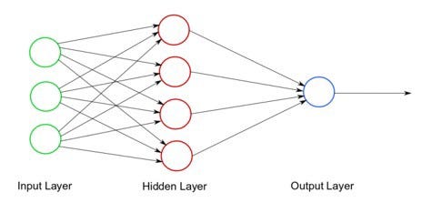
Each perceptron sends multiple signals, one signal going to each perceptron in the next layer. For each signal, the perceptron uses different weights. In the diagram above, every line going from a perceptron in one layer to the next layer represents a different output. We are not going to detail the functioning of the layers at the middle of the neural network because it is very complicated.
However, we can interest us at the input and output layers to apply a picture at a neural network. There are a few important parameters and considerations to pass an image through a network :
- Image size : input images have to be at the same size as the network. higher quality image give the model more information but require more neural network nodes and more computing power to process.
- The number of channels : grayscale image have 2 channels (black and white) and color images typically have 3 color channels (Red, Green, Blue / RGB), with colors represented in the range [0,255].
- Normalizing image : certify that all pixels have the same uniform data distribution as the network. It is possible to conduct data normalization by subtracting the mean from each pixel and then dividing the outcome by the standard deviation. Example : imagine you want to pass a RGB image. First, we substract the mean, mu (average pixel intensity across all images in the training set), from each input channel. Second, we apply a scaling factor sigma by dividing. This factor is used to scale the input image space into the particular architecture range. $$ R = (R - mur)/sigma $$$$ G = (G - mug)/sigma $$$$ B = (B - mub)/sigma $$ In lot of cases, to process an image, the value of sigma is 1 (not any scale) or 255 ( to scale the 8 bits of a picture at an interval [0 ; 1]).
When we get all this informations, an OpenCV function helps us to pass the picture in the network without calculation :
cv2.dnn.blobFromImage(image, scalefactor=1.0, size, mean, swapRB=True).
The final output (transmitted by the output layer) is a vector of probabilities, which predicts, for each feature in the image, how likely it is to belong to a class. Usually, the programmer establish a threshold parameter of prediction. If, for one feature, the final output is superior at the threshold parameter, the system signals on the output image that it has recognized something (and maybe the prediction percentage).
Different models and implementations of object detection may have different formats, but the idea is the same, which is to output the probability and the location of the object (contrary to object classification which just classifies). But, we have seen that is possible to use the sliding window to localize the image. We have also mentioned that this method is not very efficient because :
- Types of object can vary sizes ( example : small and large building).
- The ratio of height to width ( or the shapes ) of an object bounding box can be different. To solve these problems, we would have to try out different sizes/shapes of sliding window, which is very computationally intensive.
Algorithms like SSD (Single-Shot Detector) use a fully convolutional approach in which the network is able to find all objects within an image in one pass (hence ‘single-shot’). SSD has two components: a backbone model and SSD head. Backbone model usually is a pre-trained image classification network as a feature extractor.
The network I have chosen for my utilisation is MobilNet (developped by Google) because it is optimized for having a small model size and faster inference time. This is ideal to run on mobile phones and resource-constrained devices like a Rasbperry Pi. For this architecture, the backbone results in a 300x300x3 feature maps for an input image.
The SSD is a convolutional neural network which contains an output interpreted as bounding boxes surrounding classes of objects and the detection predictions associated. SSD divides the image using a grid and have each grid cell be responsible for detecting objects in that region of the image. Detection objects simply means predicting the class and location of an object within that region. If no object is present, we consider it as the background class and the location is ignored. For instance, we could use a 13x18 grid in the example below. Each grid cell is able to output the position and shape of the object it contains.

The grid system is very simple but if we need to detect multiple objects in one grid or object in different shapes we have to use anchor boxes.
Each grid cell in SSD can be assigned with multiple anchor/prior boxes. These anchor boxes are pre-defined and each one is responsible for a size and shape within a grid cell. For example, the person in the image below corresponds to the taller anchor box while the car corresponds to the wider box.

Each anchor box is specified by an aspect ratio and a zoom level.
Objects have different shapes (square, rectangle ...) and different ratios between their width and their height. The SSD architecture allows pre-defined aspect ratios of the anchor boxes. The ratios parameter can be used to specify the different aspect ratios of the anchor boxes associates with each grid cell at each zoom/scale level.
To detect an object, it is not necessary that anchor boxes and grid cells are the same size. We might be interested in finding smaller or larger objects within a grid cell. The zooms parameter is used to specify how much the anchor boxes need to be scaled up or down with respect to each grid cell. As we have seen in the grid figure below, the size of the people takes around ten grid cells but their are surround by an anchor box.
I used the SSD algorithm with a model which contains 20 classes and trained through MobilNet architecture . This 20 classes enable at the system to make differences between a man, a car, a tree, a plane ... and not just detect something. We can explain the output image by this chart :

I try to used this model for a video on the Raspberry, the device was abler to process 1 frame each 2 seconds (0.5 FPS). I retry to execute the program on the Rasbperry Pi with the NCS plugged-in, the device was able to process 6 frames per seconds ( around 10 times faster). Thanks to this experience we can appreciate the powerful of the VPU in the NCS. Thanks to this processing speed, the device is able to detect classes in "real-time" (not in real time because it stays inferior at 25 FPS but we can see beneath the video is smooth). Therefore, I try to recover a video and process a detection in the same time, it works at 6 FPS. I read in an article that with the Raspberry Pi 3+, it is possible to go until 8,5 FPS. I think it would be very interesting to test this program on a Raspberry Pi 4 equipped with a NCS.
We have seen that SSD is fast and accurate as 70% which it is not bad enough. The better type of SSD, SSD500 achieves 76.9% mAP at 22 FPS. However, this algorithm also suffers from a notable drawback : the feature does not contain enough spatial information for precise boundary generation. Therefore, it is impossible for this algorithm to detect roads.


Semantic segmentation is the task of classifying each and very pixel in an image into a class as shown in the image below. Here you can see that all persons are blue, the road is purple, the vehicles are red, sidewalk are pink .... There are three levels of image analysis :
- Classification : categorizing the entire image into a class such as “people”, “animals”, “outdoors”.
- ** Object detection ** : detecting objects within an image and drawing a rectangle around them (like SSD)
- Semantic segmentation : classifying all the pixels of an image into meaningful classes of objects. These classes are “semantically interpretable” and correspond to real-world categories.
Semantic segmentation is used for autonomous vehicles experimentations (like cars and drones) because, in comparison with object detection, it can give more accurate pixel-wise extraction results. An other reason is the fact that it is difficult to draw a bounding box surrounding the road in real-time, it is easier and more accurate to overlay a color class to highlight it.

Semantic segmentation is different from instance segmentation which is that different objects of the same class will have different labels as in person1, person2 and hence different colours. The picture below very crisply illustrates the difference between instance and semantic segmentation.

The semantic segmentation architecture I have used for my project is ENet. The reasons for why I have chosen Enet are simple : the primary benefits of ENet is that it is very fast and requiring 79x fewer parameters than larger models. I also try to use an other architecture named VGG 16, it was a little more accurate but 3x slower. In fact, with my computer, I process an image in 0,7 seconds with the Enet model and in 2,2 seconds with a VGG 16 model. With the Enet architecture model, the processing time is not nearly fast enough to make a real-time processing, so we cannot think about the possiblity of implement the VGG 16 architecture model on the Rasbperry Pi. Moreover, this last model works with the framework Keras and it is not compatible with the NCS 2.
The model chosen was trained with the Cityscape dataset which can be used for urban scene understanding. This particular model was trained with 20 classes. After processed the picture with a semantic segmentation model, I made a little program which prints the colors corresponding to classes on the picture (to help the user to interpret the image) :

When I succeeded to process one image, the next task was to process a video file. I try to use the Rasbperry Pi and the NCS to make that. i spent many time (0,7 seconds per pictures) but it worked. You can see one of my results below. I think we can be satisfy according to the result because the accuracy is not so ba, the main remaining issue is the processing time.
Thanks to the drone equipped by a camera, I have made several videos with 3 different angles of view. It is possible with the camera of the Raspberry Pi to change its angle position as you can see below :

Because the SS and the SSD models were trained with a dataset with a view angle of 0° (pedestrian view), as the camera angle of view increases, the process degrades.


With a view angle of 10°, the results are very good. There is a little bug in the SS process due to the road color. It exists also a lag in the SSD process, the process has trouble with overlapping cars.


With an angle of 45°, the results are not as good. The SS process does not detect the road. At several times, the SSD architecture the car detection with a chair. This models were not trained with this view angle and it is not able to process with accuracy this images. The last videos will confirm this theory.


With the "sentinel mode" (camera paralell to the floor), nothing is usable. To conclude to this videos, we can say that we have to train our own models (for SS and SSD architectures) with this several view angles. The training will be difficult and we have to perform it with a big dataset but this is necesary to have trustworthy models.
The objective of the project was to detect obstacles from a drone. To sump up, the system recognizes obstacles through the labels trained in the model. To realize this task, I try different techniques of computer vision. This table will sum up all this techniques and their assets :
| HAAR classifier | SSD | Semantic segmentation | |
|---|---|---|---|
| Time process (with NCS & RPI) | 3 FPS | 6 FPS | 1.5 FPS |
| Model architecture | Haar Cascade Classifiers | MobilNet | Enet |
| Global accuracy | 93% | 70% | 59,5% |
| Several classes | No | Yes | Yes |
| Bounding box | Yes | Yes | Pixel-wise |
| Compatible RPi | Yes | Yes | Yes but not adviced |
The technique the most adapted to our drone utilisation is semantic segmentation. A possibility to be more accurate for the obstacles we want to detect would be to create our own model. It can be time consuming but not a waste of time. The remaining issue is time of processing pixel by pixel. Therefore, we can look into improve the Single-Shot-Detector model by creating our own model. Maybe we have to find another architecture less adapt to the resource-constrained devices but more accurate.
To conclude, we can say that I have reached certain objectives, I have implement to machine learning models which are able to detect some obstacles on the Rasbperry Pi. Now, we have to go ahead creating our own model to detect classes we want to see. I suggest to train this model with Cityscape dataset because the drone will be drove at exterior. Meanwhile, it subsists a hardware problem because the Rasbperry Pi and the NCS will not be able to detect all classes at 20 FPS. To solve this issue of time processing, I suggest to use another single board computer. I suggest to try firstly the Raspberry Pi 4 and the NCS 2. It will be better (around 8,5 FPS) but not powerful enough to handle the real-time processing. We can check various alternative more powerful than the Raspberry Pi on this link.
For our experimentation, the drone has to be completely autonomous. To succeed in this project, the drone must detect all obstacles for any angles of view. Therefore, it is necesary to train our own models with a dataset which contains various angles.
Figure [1] : https://www.pinterest.com/pin/291959988335451420/
Figure [2] : https://www.pyimagesearch.com/wp-content/uploads/2014/10/sliding_window_example.gif
Figure [3] : https://mc.ai/using-artificial-neural-network-for-image-classification/