Snakemake workflow: sORTholog

Aim

This software will produce a table visualization of the presence or absence of encoded proteins in a given set of genomes. Both, the proteins and set of proteomes are required as input by the user.

The primary output will be the table of sORTholog protein data filled using the NCBI Protein Database, as well as PDF and PNG files of the table visualization.

Wiki page

If you need more information about some part of the sORTholog workflow please visit the Documentation Wiki page.

Installation and Running

Step 1: Install Snakemake and Snakedeploy

This pipeline uses the Snakemake workflow, that is only available on unix environment. Any linuxOS or MacOS should be able to run sORTholog. Windows users could use the workflow using the Ubuntu virtual environment.

Snakemake and Snakedeploy are best installed via the Mamba package manager (a drop-in replacement for conda). If you have neither Conda nor Mamba, it can be installed via Mambaforge. For other options see here.

To install Mamba by conda, run

conda install mamba -n base -c conda-forge

Given that Mamba is installed, run

mamba create -c bioconda -c conda-forge --name snakemake snakemake snakedeploy

to install both Snakemake and Snakedeploy in an isolated environment.

Notes

For all following commands (step 2 to 5) ensure that this environment is activated via

conda activate snakemake

⚠️ This command has to be used every single time you want to use sORTholog to be able to activate the conda environment that contains snakemake.

Step 2: Deploy workflow

Given that Snakemake and Snakedeploy are installed and available (see Step 1: install Snakemake and Snakedeploy), the workflow can be deployed as follows.

First, create an appropriate working directory, in which sORTholog will be deployed, on your system in the place of your choice as follow (note to change the path and file name to the one you want to create):

mkdir path/to/sORTholog

Then go to your sORTholog working directory as follow:

cd path/to/sORTholog

Second, run (if your are in the sORTholog directory)

snakedeploy deploy-workflow https://github.com/vdclab/sORTholog . --tag 0.6.2

else, run

snakedeploy deploy-workflow https://github.com/vdclab/sORTholog path/to/sORTholog --tag 0.6.2

Snakedeploy will create two folders workflow and config. The former contains the deployment of the chosen workflow as a Snakemake module, the latter contains configuration files which will be modified in the next step in order to configure the workflow to your needs. Later, when executing the workflow, Snakemake will automatically find the main Snakefile in the workflow subfolder.

Step 3: Configure workflow

The three files described in this section (Taxids file, Seeds file, and Config file) can be edited with a text editor.

Taxids file

The taxid file is a table, in the format of a tabulated text file (e.g. .txt, .tsv). This table should contain 2 columns: TaxId and NCBIGroups. The TaxId columns should be filled with the TaxId of the genome you want to analyze. You can use any clade TaxId, sORTholog will take care of downloading all the genome of this clade. The NCBIGroups can be left blanked, but knowing this group would make the download of genomes faster. Here a list of accepted terms: all, archaea, bacteria, fungi, invertebrate, metagenomes, plant, protozoa, vertebrate_mammalian, vertebrate_other, viral. This will allow to look in the right folder in the FTP of NCBI to download the proteome. By choosing all, it will look in all folders and slow down the process. Ideally your taxid file should be in your sORTholog working directory or in the config folder. Example provided in the file doc/dummy_taxids.tsv folder in the GitHub page.

Seeds file

The seed file contains the list of proteins you want to identify in your genomes. It is a table, in the format of a tabulated text file (e.g. .txt, .tsv). Ideally your seed file should be in your workdir folder or in the config folder.

Here is a list of collumns for this file:

• seed: Mandatory, name of the protein as you want it to appear in the final figure.
• protein_id: Mandatory, either the NCBI protein id of a protein you are sure have the function you are searching for.
• hmm: name of the hmm profile file associated with the protein family, including the extension, often .hmm. (no default, if not mentioned, psiBLAST will be triggered instead)
• evalue: Number between 0 and 1, e-value threshold of blast.
• pident: Number between 0 and 1, percentage of identity (expressed in frequency) threshold of blast.
• cov: Number between 0 and 1, coverage threshold (expressed in frequency) for blast results. The coverage is based on the coverage of the query.
• color: hexadecimal code of the color you want the positive results to be in the final figure for this seed.

Example provided in the file doc/dummy_seeds.tsv folder in the GitHub page.

Common mistakes

• Columns in the seed files should be separated by tabulation, introduction of spaces or other hidden characters might disrupt the reading of the file.
• Do not introduce empty lines in the seed file.
• Make sure to have the correct extension for your hmm profile.

A detail explaination of the config file is available in the wiki in How to Install and Set Up sORTholog

Step 4: Run the workflow

Given that the workflow has been properly deployed and configured, it can be executed as follows.

For running the workflow while deploying any necessary software via conda, run Snakemake with

snakemake --cores 1 --use-conda 

Here the number of used for the workflow is set to 1 but the number could be increase if needed.

If you want to run the workflow with the additional step to speedup the analysis that contains a big dataset you can either:

• Change in the config.yaml the parameter speedup and change the value to True
• Run the workflow adding -C speedup=True to the command line as follow

snakemake --cores 1 --use-conda -C speedup=True

You will find the table of presence of absence patab_table.tsv, the melt version of this table patab_melt.tsv and a folder plots containing the figure representing the table.

Step 5: Generate report

After finalizing your data analysis, you can automatically generate an interactive visual HTML report for inspection of results together with parameters and code inside of the browser via

snakemake --report report.zip --report-stylesheet config/report.css

The resulting report.zip file can be passed on to collaborators, provided as a supplementary file in publications.

Important Notes for running on the UFL cluster

If you want to run the workflow on the UFL cluster please follow the gideline in the Wiki part: 3b Running sORTholog cluster

Walk-Through and File Production

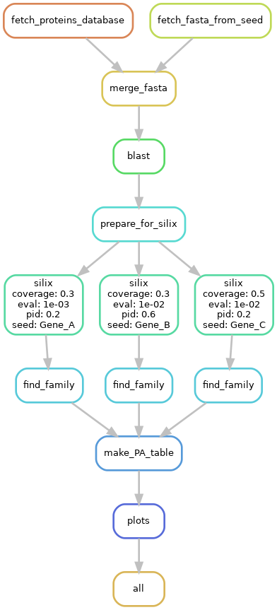
This pipeline consists of 9/12 steps called rules that take input files and create output files. Here is a description of the pipeline.

1. As snakemake is set up, there is a last rule, called all, that serves to call the last output files and make sure they were created.

2. A folder containing your work will be created:

   [project_name]/                           <- top-level project folder (your project_name)
   │
   │
   ├── report.html                           <- This report file      
   │
   ├── logs                                  <- Collection of log outputs, e.g. from cluster managers
   │
   ├── databases                             <- Generated analysis database related files
   │   ├── all_taxid                         
   │   │   ├─ protein_table.tsv              <- Table with the informations about the proteins of the downloaded taxid
   │   │   ├─ summary_assembly_taxid.tsv     <- Table with the informations about the downloaded genome from NCBI
   │   │   ├─ taxid_all_together.fasta       <- Fasta file of the downloaded taxid
   │   │   └─ taxid_checked.txt              <- List of the downloaded taxid
   │   │
   │   ├── merge_fasta                       
   │   │   └─ taxid_checked.txt              <- Fasta with the concatenation of the genome of interest and seeds
   │   │
   │   └── seeds                             
   │       ├─ seeds.fasta                    <- Fasta file of the seeds
   │       └─ new_seeds.tsv                  <- Table with the informations about the seeds
   │
   ├── analysis_thresholds                   <- (Optional) Generate by the rule report_thresholds
   │   ├── tables                         
   │   │   └─ table--seed.tsv                <- (Optional) Table with the information of each pair of hits in for the seed family (one per seed)
   │   │
   │   └── report_figure_thresholds.html     <- (Optional) HTML report with the plots made by report_thresholds                  
   │
   └── results                               <- Final results for sharing with collaborators, typically derived from analysis sets
       ├── fasta                             <- (Optional) folder with the fasta file of the orthologs of the seeds
       ├── patab_melt.tsv                    <- Table with the information of sORTholog one information by line
       ├── patab_table.tsv                   <- Table with the information of presence absence with genome in index and seeds in columns and proteins Id in the cell
       └── plots                             <- Plots and table on which the plot are created

3. Before starting the pipeline, your taxids will be checked and updated for the lowest descendant levels. This will create a file of checked taxids. It will skip this step if this file already exists.

4. When restarting the pipeline, the software will check if you made any changes in the seed file before running. If changes have been made, it will run what is necessary, else nothing will happen.

Pipeline in image

Only blast and silix behavior

Speedup behavior