These implementations are for demonstration purposes. They are less efficient than the implementations in the Python standard library.
Bubble sort, sometimes referred to as sinking sort, is a simple sorting algorithm that repeatedly steps through the list to be sorted, compares each pair of adjacent items and swaps them if they are in the wrong order. The pass through the list is repeated until no swaps are needed, which indicates that the list is sorted.
Properties
- Worst case performance O(n2)
- Best case performance O(n)
- Average case performance O(n2)
Source: Wikipedia
View the algorithm in action
Bucket sort, or bin sort, is a sorting algorithm that works by distributing the elements of an array into a number of buckets. Each bucket is then sorted individually, either using a different sorting algorithm, or by recursively applying the bucket sorting algorithm.
Properties
- Worst case performance O(n2)
- Best case performance O(n+k)
- Average case performance O(n+k)
Source: Wikipedia
Cocktail shaker sort, also known as bidirectional bubble sort, cocktail sort, shaker sort (which can also refer to a variant of selection sort), ripple sort, shuffle sort, or shuttle sort, is a variation of bubble sort that is both a stable sorting algorithm and a comparison sort. The algorithm differs from a bubble sort in that it sorts in both directions on each pass through the list.
Properties
- Worst case performance O(n2)
- Best case performance O(n)
- Average case performance O(n2)
Source: Wikipedia
Insertion sort is a simple sorting algorithm that builds the final sorted array (or list) one item at a time. It is much less efficient on large lists than more advanced algorithms such as quicksort, heapsort, or merge sort.
Properties
- Worst case performance O(n2)
- Best case performance O(n)
- Average case performance O(n2)
Source: Wikipedia
View the algorithm in action
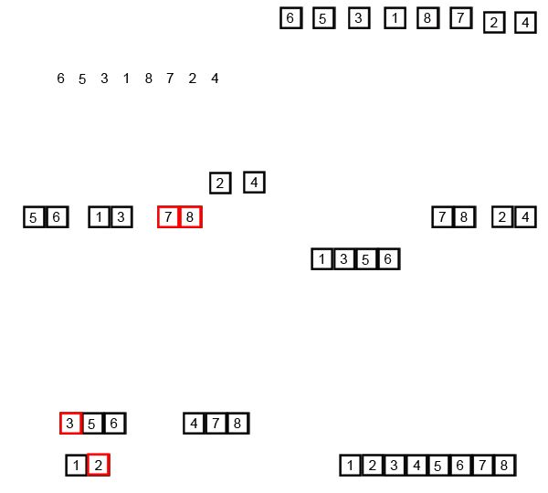
Merge sort (also commonly spelled mergesort) is an efficient, general-purpose, comparison-based sorting algorithm. Most implementations produce a stable sort, which means that the implementation preserves the input order of equal elements in the sorted output. Mergesort is a divide and conquer algorithm that was invented by John von Neumann in 1945.
Properties
- Worst case performance O(n log n)
- Best case performance O(n log n)
- Average case performance O(n log n)
Source: Wikipedia
View the algorithm in action
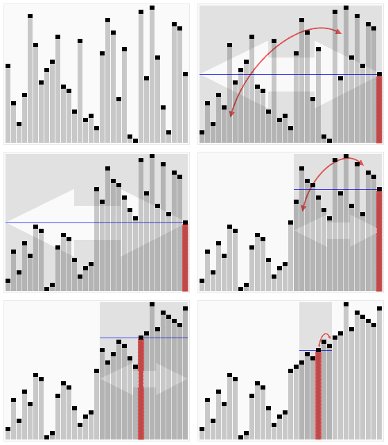
Quicksort (sometimes called partition-exchange sort) is an efficient sorting algorithm, serving as a systematic method for placing the elements of an array in order.
Properties
- Worst case performance O(n2)
- Best case performance O(n log n) or O(n) with three-way partition
- Average case performance O(n log n)
Source: Wikipedia
View the algorithm in action
Heapsort is a comparison-based sorting algorithm. It can be thought of as an improved selection sort. It divides its input into a sorted and an unsorted region, and it iteratively shrinks the unsorted region by extracting the largest element and moving that to the sorted region.
Properties
- Worst case performance O(n log n)
- Best case performance O(n log n)
- Average case performance O(n log n)
Source: Wikipedia
View the algorithm in action
From Wikipedia: Radix sort is a non-comparative integer sorting algorithm that sorts data with integer keys by grouping keys by the individual digits which share the same significant position and value.
Properties
- Worst case performance O(wn)
- Best case performance O(wn)
- Average case performance O(wn)
Source: Wikipedia
Selection sort is an algorithm that divides the input list into two parts: the sublist of items already sorted, which is built up from left to right at the front (left) of the list, and the sublist of items remaining to be sorted that occupy the rest of the list. Initially, the sorted sublist is empty and the unsorted sublist is the entire input list. The algorithm proceeds by finding the smallest (or largest, depending on sorting order) element in the unsorted sublist, exchanging (swapping) it with the leftmost unsorted element (putting it in sorted order), and moving the sublist boundaries one element to the right.
Properties
- Worst case performance O(n2)
- Best case performance O(n2)
- Average case performance O(n2)
Source: Wikipedia
View the algorithm in action
Shellsort is a generalization of insertion sort that allows the exchange of items that are far apart. The idea is to arrange the list of elements so that, starting anywhere, considering every nth element gives a sorted list. Such a list is said to be h-sorted. Equivalently, it can be thought of as h interleaved lists, each individually sorted.
Properties
- Worst case performance O(nlog2n)
- Best case performance O(n log n)
- Average case performance depends on gap sequence
Source: Wikipedia
View the algorithm in action
From Wikipedia: Topological sort, or topological ordering of a directed graph is a linear ordering of its vertices such that for every directed edge uv from vertex u to vertex v, u comes before v in the ordering. For instance, the vertices of the graph may represent tasks to be performed, and the edges may represent constraints that one task must be performed before another; in this application, a topological ordering is just a valid sequence for the tasks. A topological ordering is possible if and only if the graph has no directed cycles, that is, if it is a directed acyclic graph (DAG). Any DAG has at least one topological ordering, and algorithms are known for constructing a topological ordering of any DAG in linear time.
Comparing the complexity of sorting algorithms (Bubble Sort, Insertion Sort, Selection Sort)
Comparing the sorting algorithms:
-Quicksort is a very fast algorithm but can be pretty tricky to implement
-Bubble sort is a slow algorithm but is very easy to implement. To sort small sets of data, bubble sort may be a better option since it can be implemented quickly, but for larger datasets, the speedup from quicksort might be worth the trouble implementing the algorithm.
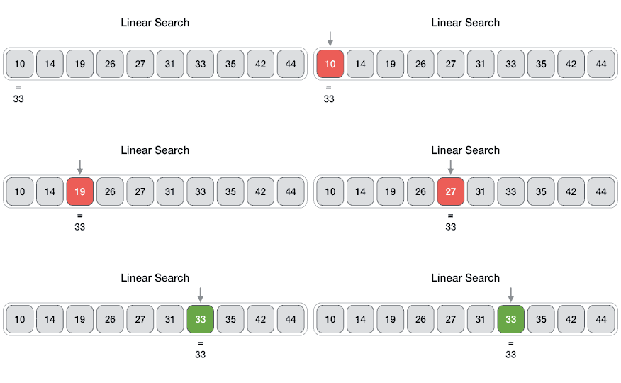
Linear search or sequential search is a method for finding a target value within a list. It sequentially checks each element of the list for the target value until a match is found or until all the elements have been searched. Linear search runs in at worst linear time and makes at most n comparisons, where n is the length of the list.
Properties
- Worst case performance O(n)
- Best case performance O(1)
- Average case performance O(n)
- Worst case space complexity O(1) iterative
Source: Wikipedia
Binary search, also known as half-interval search or logarithmic search, is a search algorithm that finds the position of a target value within a sorted array. It compares the target value to the middle element of the array; if they are unequal, the half in which the target cannot lie is eliminated and the search continues on the remaining half until it is successful.
Properties
- Worst case performance O(log n)
- Best case performance O(1)
- Average case performance O(log n)
- Worst case space complexity O(1)
Source: Wikipedia
Interpolation search is an algorithm for searching for a key in an array that has been ordered by numerical values assigned to the keys (key values). It was first described by W. W. Peterson in 1957. Interpolation search resembles the method by which people search a telephone directory for a name (the key value by which the book's entries are ordered): in each step the algorithm calculates where in the remaining search space the sought item might be, based on the key values at the bounds of the search space and the value of the sought key, usually via a linear interpolation. The key value actually found at this estimated position is then compared to the key value being sought. If it is not equal, then depending on the comparison, the remaining search space is reduced to the part before or after the estimated position. This method will only work if calculations on the size of differences between key values are sensible.
By comparison, binary search always chooses the middle of the remaining search space, discarding one half or the other, depending on the comparison between the key found at the estimated position and the key sought — it does not require numerical values for the keys, just a total order on them. The remaining search space is reduced to the part before or after the estimated position. The linear search uses equality only as it compares elements one-by-one from the start, ignoring any sorting.
On average the interpolation search makes about log(log(n)) comparisons (if the elements are uniformly distributed), where n is the number of elements to be searched. In the worst case (for instance where the numerical values of the keys increase exponentially) it can make up to O(n) comparisons.
In interpolation-sequential search, interpolation is used to find an item near the one being searched for, then linear search is used to find the exact item.
Source: Wikipedia
Jump search or block search refers to a search algorithm for ordered lists. It works by first checking all items Lkm, where {\displaystyle k\in \mathbb {N} } k\in \mathbb {N} and m is the block size, until an item is found that is larger than the search key. To find the exact position of the search key in the list a linear search is performed on the sublist L[(k-1)m, km].
The optimal value of m is √n, where n is the length of the list L. Because both steps of the algorithm look at, at most, √n items the algorithm runs in O(√n) time. This is better than a linear search, but worse than a binary search. The advantage over the latter is that a jump search only needs to jump backwards once, while a binary can jump backwards up to log n times. This can be important if a jumping backwards takes significantly more time than jumping forward.
The algorithm can be modified by performing multiple levels of jump search on the sublists, before finally performing the linear search. For an k-level jump search the optimum block size ml for the lth level (counting from 1) is n(k-l)/k. The modified algorithm will perform k backward jumps and runs in O(kn1/(k+1)) time.
Source: Wikipedia
Quick Select is a selection algorithm to find the kth smallest element in an unordered list. It is related to the quicksort sorting algorithm. Like quicksort, it was developed by Tony Hoare, and thus is also known as Hoare's selection algorithm.[1] Like quicksort, it is efficient in practice and has good average-case performance, but has poor worst-case performance. Quickselect and its variants are the selection algorithms most often used in efficient real-world implementations.
Quickselect uses the same overall approach as quicksort, choosing one element as a pivot and partitioning the data in two based on the pivot, accordingly as less than or greater than the pivot. However, instead of recursing into both sides, as in quicksort, quickselect only recurses into one side – the side with the element it is searching for. This reduces the average complexity from O(n log n) to O(n), with a worst case of O(n2).
As with quicksort, quickselect is generally implemented as an in-place algorithm, and beyond selecting the k'th element, it also partially sorts the data. See selection algorithm for further discussion of the connection with sorting.
Source: Wikipedia
Tabu search uses a local or neighborhood search procedure to iteratively move from one potential solution {\displaystyle x} x to an improved solution {\displaystyle x'} x' in the neighborhood of {\displaystyle x} x, until some stopping criterion has been satisfied (generally, an attempt limit or a score threshold). Local search procedures often become stuck in poor-scoring areas or areas where scores plateau. In order to avoid these pitfalls and explore regions of the search space that would be left unexplored by other local search procedures, tabu search carefully explores the neighborhood of each solution as the search progresses. The solutions admitted to the new neighborhood, {\displaystyle N^{}(x)} N^(x), are determined through the use of memory structures. Using these memory structures, the search progresses by iteratively moving from the current solution {\displaystyle x} x to an improved solution {\displaystyle x'} x' in {\displaystyle N^{}(x)} N^(x).
These memory structures form what is known as the tabu list, a set of rules and banned solutions used to filter which solutions will be admitted to the neighborhood {\displaystyle N^{}(x)} N^(x) to be explored by the search. In its simplest form, a tabu list is a short-term set of the solutions that have been visited in the recent past (less than {\displaystyle n} n iterations ago, where {\displaystyle n} n is the number of previous solutions to be stored — is also called the tabu tenure). More commonly, a tabu list consists of solutions that have changed by the process of moving from one solution to another. It is convenient, for ease of description, to understand a “solution” to be coded and represented by such attributes.
Source: Wikipedia
![alt text][caesar]
Caesar cipher, also known as Caesar's cipher, the shift cipher, Caesar's code or Caesar shift, is one of the simplest and most widely known encryption techniques.
It is a type of substitution cipher in which each letter in the plaintext is replaced by a letter some fixed number of positions down the alphabet. For example, with a left shift of 3, D would be replaced by A, E would become B, and so on.
The method is named after Julius Caesar, who used it in his private correspondence.
The encryption step performed by a Caesar cipher is often incorporated as part of more complex schemes, such as the Vigenère cipher, and still has modern application in the ROT13 system. As with all single-alphabet substitution ciphers, the Caesar cipher is easily broken and in modern practice offers essentially no communication security.
Source: Wikipedia
Vigenère cipher is a method of encrypting alphabetic text by using a series of interwoven Caesar ciphers based on the letters of a keyword. It is a form of polyalphabetic substitution.
The Vigenère cipher has been reinvented many times. The method was originally described by Giovan Battista Bellaso in his 1553 book La cifra del. Sig. Giovan Battista Bellaso; however, the scheme was later misattributed to Blaise de Vigenère in the 19th century, and is now widely known as the "Vigenère cipher".
Though the cipher is easy to understand and implement, for three centuries it resisted all attempts to break it; this earned it the description le chiffre indéchiffrable(French for 'the indecipherable cipher').
Many people have tried to implement encryption schemes that are essentially Vigenère ciphers. Friedrich Kasiski was the first to publish a general method of deciphering a Vigenère cipher in 1863.
Source: Wikipedia
Transposition cipher is a method of encryption by which the positions held by units of plaintext (which are commonly characters or groups of characters) are shifted according to a regular system, so that the ciphertext constitutes a permutation of the plaintext. That is, the order of the units is changed (the plaintext is reordered).
Mathematically a bijective function is used on the characters' positions to encrypt and an inverse function to decrypt.
Source: Wikipedia
RSA (Rivest–Shamir–Adleman) is one of the first public-key cryptosystems and is widely used for secure data transmission. In such a cryptosystem, the encryption key is public and it is different from the decryption key which is kept secret (private). In RSA, this asymmetry is based on the practical difficulty of the factorization of the product of two large prime numbers, the "factoring problem". The acronym RSA is made of the initial letters of the surnames of Ron Rivest, Adi Shamir, and Leonard Adleman, who first publicly described the algorithm in 1978. Clifford Cocks, an English mathematician working for the British intelligence agency Government Communications Headquarters (GCHQ), had developed an equivalent system in 1973, but this was not declassified until 1997.[1]
A user of RSA creates and then publishes a public key based on two large prime numbers, along with an auxiliary value. The prime numbers must be kept secret. Anyone can use the public key to encrypt a message, but with currently published methods, and if the public key is large enough, only someone with knowledge of the prime numbers can decode the message feasibly.[2] Breaking RSA encryption is known as the RSA problem. Whether it is as difficult as the factoring problem remains an open question.
Source: Wikipedia
ROT13 ("rotate by 13 places", sometimes hyphenated ROT-13) is a simple letter substitution cipher that replaces a letter with the 13th letter after it, in the alphabet. ROT13 is a special case of the Caesar cipher which was developed in ancient Rome.
Because there are 26 letters (2×13) in the basic Latin alphabet, ROT13 is its own inverse; that is, to undo ROT13, the same algorithm is applied, so the same action can be used for encoding and decoding. The algorithm provides virtually no cryptographic security, and is often cited as a canonical example of weak encryption.[1]
Source: Wikipedia
XOR cipher is a simple type of additive cipher,[1] an encryption algorithm that operates according to the principles:
A {\displaystyle \oplus } \oplus 0 = A, A {\displaystyle \oplus } \oplus A = 0, (A {\displaystyle \oplus } \oplus B) {\displaystyle \oplus } \oplus C = A {\displaystyle \oplus } \oplus (B {\displaystyle \oplus } \oplus C), (B {\displaystyle \oplus } \oplus A) {\displaystyle \oplus } \oplus A = B {\displaystyle \oplus } \oplus 0 = B, where {\displaystyle \oplus } \oplus denotes the exclusive disjunction (XOR) operation. This operation is sometimes called modulus 2 addition (or subtraction, which is identical).[2] With this logic, a string of text can be encrypted by applying the bitwise XOR operator to every character using a given key. To decrypt the output, merely reapplying the XOR function with the key will remove the cipher.


