More with CSP

Nodes in csp have many more complex features than we saw in the First Steps example. These include state, alarms and start/stop execution blocks. Also, the csp library has an extensive set of pre-written nodes that are optimized in C++. You can leverage these nodes to quickly build high-performing applications.

In this tutorial, you will create a Poisson counter that counts the number of events in a Poisson process. We will then look at the correlation between two independent Poisson processes by leveraging nodes in baselib and stats.

Building our Poisson counter

A Poisson point process has events which are exponentially distributed across time. The average delay between events is controlled by the rate parameter "rate". In the poisson_counter node below, we use the following useful node features:

1. csp.state: we keep a state variable in the node which is the count of events thus far. A state variable can be thought of as a "member" of the node.
2. csp.alarms: we schedule an alarm to simulate each event. An alarm is an internal time series which feeds back to the same node.
3. csp.start: we schedule the first alarm at start time, which is when the graph begins execution. There is also a stop block available in nodes which runs when the graph stops.

We also turn off memoization for the node by passing memoize=False. This means that when we create two poisson_counter nodes with the same "rate" argument we get two different random time series.

import csp
from csp import ts
from datetime import timedelta
import numpy as np

@csp.node(memoize=False)
def poisson_counter(rate: float) -> ts[int]:
    with csp.alarms():
        event = csp.alarm(int)
    with csp.state():
        s_count = 0
    with csp.start():
        delay = np.random.exponential(rate)
        csp.schedule_alarm(event, timedelta(seconds=delay), True)
        
    if csp.ticked(event):
        s_count += 1
        next_delay = np.random.exponential(rate)
        csp.schedule_alarm(event, timedelta(seconds=next_delay), True)
        return s_count

We can run the node using csp.run as follows:

from datetime import datetime

res = csp.run(poisson_counter, rate=2.0, starttime=datetime.utcnow(), endtime=timedelta(seconds=10), realtime=False)
print(f'Final count: {res[0][-1][1]}')

Since the rate is set to 2.0, we would expect a new event approximately every 2.0 seconds. Therefore, the average of multiple runs should converge to 5 events. Running the counter multiple times, we get:

Final count: 6
Final count: 1
Final count: 6
Final count: 5
Final count: 5
Final count: 2
Final count: 9
...

Correlation between two Poisson processes

We can use a combination of pre-written nodes from baselib and stats to calculate the correlation of two Poisson point processes in 1-minute buckets. Even though both processes have the same rate they will be fully independent, so we expect the correlation to converge to zero.

We will first compute the number of events in each 1-minute period by using the (csp.diff)[Base-Nodes-API#cspdiff] and (csp.sample)[Base-Nodes-API#cspsample] functions. diff gives the difference between the value of a time series at the current time and some time in the past. sample will get the value of a time series whenever some other time series ticks. We will also use a (csp.timer)[Base-Adapters-API#csptimer] so that we sample the values every minute.

@csp.graph
def events_per_minute_bucket(poisson_counter: ts[int]) -> ts[int]:
    minute_timer = csp.timer(interval=timedelta(minutes=1), value=True)
    sampled_event_count = csp.sample(trigger=minute_timer, x=poisson_counter)
    events_per_minute = csp.diff(sampled_event_count, lag=timedelta(minutes=1))
    return events_per_minute

We can call this subgraph with two different Poisson processes of rate=1.0 to generate our 1-minute event counts. We can then find the correlation between the two series using csp.stats.corr.

from csp import stats

@csp.graph
def corr_graph() -> ts[float]:
    # Define two Poisson point processes
    process_A = poisson_counter(rate=1.0)
    process_B = poisson_counter(rate=1.0)
   
    # Get the per minute event counts
    counts_A = events_per_minute_bucket(process_A)
    counts_B = events_per_minute_bucket(process_B)

    # Compute correlation between two independent processes
    corr = csp.stats.corr(counts_A, counts_B)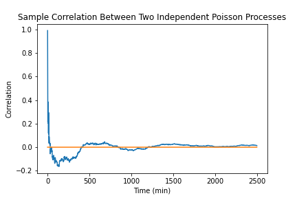
    return corr

Running the graph and analyzing results

We can run the above corr_graph for 2500 minutes of simulated time and analyze the correlation. Using:

csp.run(corr_graph, starttime=datetime(2020,1,1), endtime=timedelta(minutes=2500), realtime=False)

and extracting the correlation values, we see that the correlation converges to near zero as we expected.

Visualization

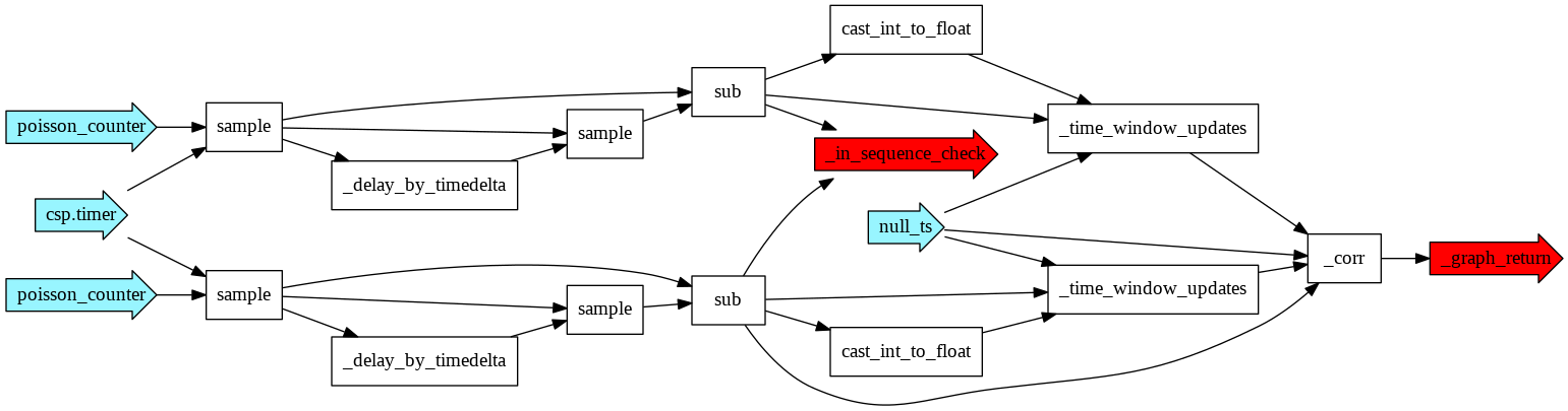
We can visualize the graph used to calculate our autocorrelation using the show_graph utility. Take a moment and match each node to where it lies in the corr_graph code. Note that many of the nodes shown are subcomponents of the library functions we used.