Time Domain Simulation
A simple LC tank circuit is used to demonstrate the usage of the transient simulation box. Also simple equations are used to predict the expected result and based on these results parameters of time domain simulation are setup.
For time domain simulation a parallel LC resonance circuit is chosen as depicted in the below figure.

We have there an inductor with L=10nH and a capacitor with C=1uF in parallel. The unknown node has been named "out" and the other node has been set to ground.
In order to see the circuit in action an excitation is required. In the below figure a DC voltage source and a resistor in series is feed to the "out" node via a time switch.

The time switch can be found in the "Components" tab in the "lumped components" category. The time switch has been chosen to be initially closed (init=on) and open at 1us.
The resonance frequency of the LC tank is meant to be
<math>f_{res} = \frac{1}{2\pi\cdot\sqrt{L\cdot C}} \approx 1.6\rm{MHz}</math>
Initially during the period when the switch is closed a DC current flows through the voltage source, the resistor and the tanks inductor. The current through this tank inductor computes as
<math>I_L = \frac{1V}{0.1\Omega} = 10\rm{A}</math>
After the switch has been opened the LC tank is meant to store energy persisting in the inductor previously by oscillating at the resonance frequency. The voltage drop across the inductor then calculates as
<math>V_L = \omega\cdot L = 2\pi\cdot f_{res}\cdot L = 1\rm{V}</math>
These hand calculations have been typed into equations on the schematic as shown in the next figure.
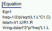
The equations demonstrate how to use component property values in schematic equations.
In order to simulate the circuit in the time domain a transient simulation box is required. It can be found in the "Components" tab in the "simulations" category.

From hand calculations it is expected that the LC tank oscillates at 1.6MHz. Thus in the transient simulation box a stop time of 10us is chosen. Thus approximately 15 cycles of the oscillation will be seen. The number of simulation steps is sufficiently high (here 400) chosen in order to see a smooth waveform.
After the simulation has been started a tabular diagram is used to display the hand calculation results and a cartesian diagram to display the voltage waveform at the node "out".

The hand calculation formulaes can be verified to be correct. In the waveform plot it can be seen that voltage keeps zero as long as the switch is closed up to 1us. With the switch opened after 1us the LC tank starts oscillating with the precalculated frequency and amplitude.
Original author: Stefan Jahn (2009)