The convdistr package

John J. Aponte

The convdistr package provide tools to define distribution objects and make mathematical operations with them. It keep track of the results as if they where scalar numbers but maintaining the ability to obtain randoms samples of the convoluted distributions.

To install this package from github

devtools::install_github("johnaponte/convdistr", build_manual = T, build_vignettes = T)

Practical example

What would be the resulting distribution of a + b * c if a is a normal distribution with mean 1 and standard deviation 0.5, b is a poisson distribution with lambda 5 and c is a beta distribution with shape parameters 10 and 20?

library(convdistr)
library(ggplot2)

a <- new_NORMAL(1,0.5)
b <- new_POISSON(5)
c <- new_BETA(10,20)
res <- a + b * c

metadata(res) 
#>   distribution     rvar
#> 1  CONVOLUTION 2.666667
summary(res)

distribution	varname	oval	nsample	mean_	sd_	lci_	median_	uci_
CONVOLUTION	rvar	2.67	10000	2.66	1.02	0.94	2.56	4.95

ggDISTRIBUTION(res) + ggtitle("a + b * c")

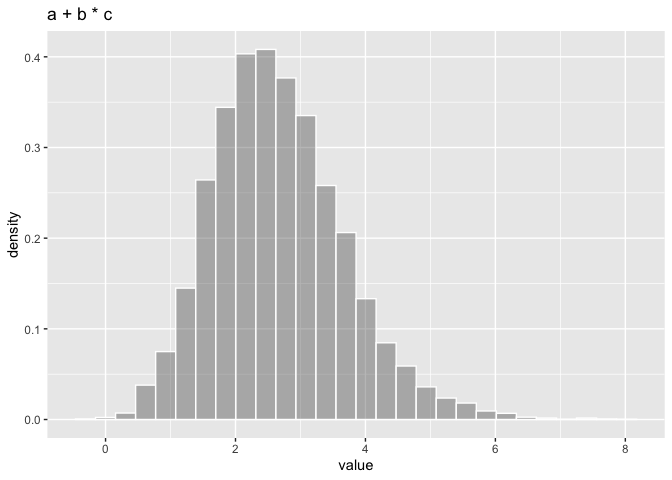
The result is a distribution with expected value 2.67. A sample from 10000 drawns of the distribution shows a mean value of 2.66, a median of 2.56 and 95% quantiles of 0.94, 4.95

The following sections describe the DISTRIBUTION object, how to create new DISTRIBUTION objects and how to make operations and mixtures with them.

Please note that when convoluting distributions, this package assumes the distributions are independent between them, i.e. their correlation is 0. If not, you need to implement specific distributions to handle the correlation, like the MULTIVARIATE object.

Description of the DISTRIBUTION object

The DISTRIBUTION is kind of abstract class (or interface) that specific constructors should implement.

It contains 4 fields:

distribution : A character with the name of the distribution implemented

seed : A numerical seed that is use to get a repeatable sample in the summary function

oval : The observed value. It is the value expected. It is used as a number for the mathematical operations of the distributions as if they were a simple scalar

rfunc(n) : A function that generate random numbers from the distribution. Its only parameter n is the number of drawns of the distribution. It returns a matrix with as many rows as n, and as many columns as the dimensions of the distributions

The DISTRIBUTION object can support multidimensional distributions for example a dirichlet distribution. The names of the dimensions should coincides with the names of the oval vector. If it has only one dimension, the default name is rvar.

It is expected that the rfunc could be included in the creation of new distributions by convolution or mixture, so the environment should be carefully controlled to avoid reference leaking that is possible within the R language. For that reason, the rfunc should be created within a restrict_environment function that controls that only the variables that are required within the function are saved in the environment of the function.

Once the new objects are instanced, the fields are immutable and should not be changed.

Factory of DISTRIBUTION objects

The following functions create new objects of class DISTRIBUTION

Distribution	factory	parameters	function
uniform	new_UNIFORM	p_min, p_max	runif
normal	new_NORMAL	p_mean, p_sd	rnorm
beta	new_BETA	p_shape1, p_shape2	rbeta
beta	new_BETA_lci	p_mean, p_lci, p_uci	rbeta
triangular	new_TRIANGULAR	p_min, p_max, p_mode	rtriangular
poisson	new_POISSON	p_lambda	rpoisson
exponential	new_EXPONENTIAL	p_rate	rexp
discrete	new_DISCRETE	p_supp, p_prob	sample
dirichlet	new_DIRICHLET	p_alpha, p_dimnames	rdirichlet
truncated	new_TRUNCATED	p_distribution, p_min, p_max
dirac	new_DIRAC	p_value
NA	new_NA	p_dimnames

Methods

The following are methods for all objects of class DISTRIBUTION

• metadata(x) Print the metadata for the distribution
• summary(object, n=10000) Produce a summary of the distribution
• rfunc(x, n) Generate n random drawns of the distribution
• plot(x, n= 10000) Produce a density plot of the distribution
• ggDISTRIBUTION(x, n= 10000) produce a density plot of the distribution using ggplot2

myDistr <- new_NORMAL(0,1)
metadata(myDistr)
#>   distribution rvar
#> 1       NORMAL    0
rfunc(myDistr, 10)
#>            rvar
#> 1  -0.202292246
#> 2   2.359176819
#> 3  -0.378977974
#> 4  -1.108465547
#> 5   0.080081266
#> 6  -0.001522165
#> 7   1.140359435
#> 8   0.220586273
#> 9   0.533860090
#> 10  1.450453816
summary(myDistr)

distribution	varname	oval	nsample	mean_	sd_	lci_	median_	uci_
NORMAL	rvar	0	10000	0.01	1.01	-1.98	0.02	1.97

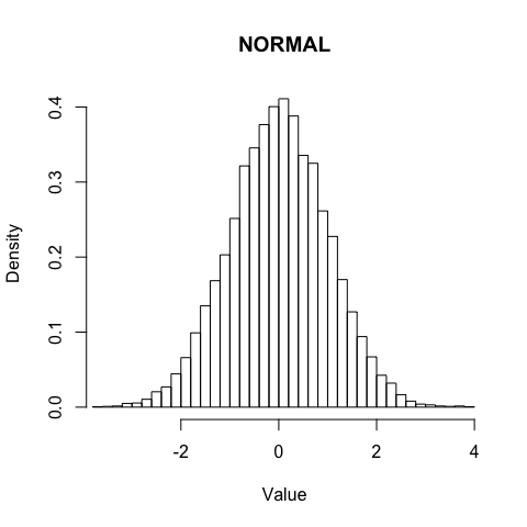
plot(myDistr)

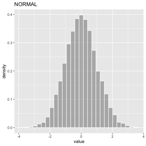
ggDISTRIBUTION(myDistr)

Convolution for Distribution with the same dimensions

Mathematical operations like +, -, *, / between DISTRIBUTION with the same dimensions can be perform with the new_CONVOLUTION(listdistr, op, omit_NA = FALSE) function. The listdistr parameter is a list of DISTRIBUTION objects on which the operation is made. A shorter version exists for each one of the operations as follow

• new_SUM(listdistr, omit_NA = FALSE)
• new_SUBTRACTION(listdistr, omit_NA = FALSE)
• new_MULTIPLICATION(listdistr, omit_NA = FALSE)
• new_DIVISION(listdistr, omit_NA = FALSE)

but Mathematical operator can also be used.

d1 <- new_NORMAL(1,1)
d2 <- new_UNIFORM(2,8)
d3 <- new_POISSON(5)
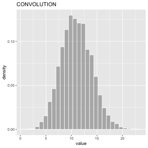
dsum <- new_SUM(list(d1,d2,d3))
dsum
#>   distribution rvar
#> 1  CONVOLUTION   11
d1 + d2 + d3
#>   distribution rvar
#> 1  CONVOLUTION   11
summary(dsum)

distribution	varname	oval	nsample	mean_	sd_	lci_	median_	uci_
CONVOLUTION	rvar	11	10000	11	3.01	5.4	10.88	17.2

ggDISTRIBUTION(dsum)

Mixture

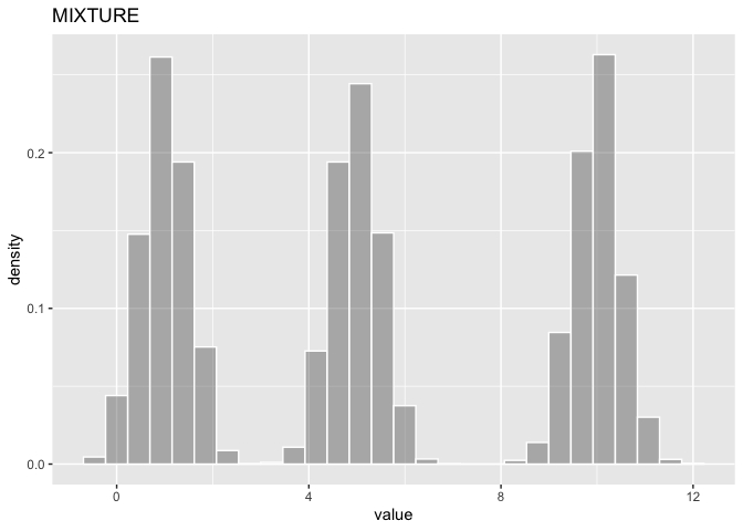
A DISTRIBUTION, consisting on the mixture of several distribution can be obtained with the new_MIXTURE(listdistr, mixture) function where listdistr is a list of DISTRIBUTION objects and mixture the vector of probabilities for each distribution. If missing the mixture, the probability will be the same for each distribution.

d1 <- new_NORMAL(1,0.5)
d2 <- new_NORMAL(5,0.5)
d3 <- new_NORMAL(10,0.5)
dmix <- new_MIXTURE(list(d1,d2,d3))
summary(dmix)

distribution	varname	oval	nsample	mean_	sd_	lci_	median_	uci_
MIXTURE	rvar	5.33	10000	5.32	3.7	0.27	4.99	10.71

ggDISTRIBUTION(dmix)

Convolution of distributions with different dimensions

When convoluting distribution with different dimensions, there are two possibilities. The new_CONVOLUTION_assoc family of functions perform the operation only on the common dimensions and left the others dimensions as they are, or the new_CONVOLUTION_comb family of functions which perform the operation in the combination of all dimensions.

d1 <- new_MULTINORMAL(c(0,1), matrix(c(1,0.3,0.3,1), ncol = 2), p_dimnames = c("A","B"))
d2 <- new_MULTINORMAL(c(3,4), matrix(c(1,0.3,0.3,1), ncol = 2), p_dimnames = c("B","C"))
summary(d1)

distribution	varname	oval	nsample	mean_	sd_	lci_	median_	uci_
MULTINORMAL	A	0	10000	0	1	-1.96	0.01	1.95
MULTINORMAL	B	1	10000	1	1	-0.95	1.00	2.94

summary(d2)

distribution	varname	oval	nsample	mean_	sd_	lci_	median_	uci_
MULTINORMAL	B	3	10000	3.01	1.00	1.04	3.03	4.97
MULTINORMAL	C	4	10000	4.01	1.01	2.04	4.00	6.00

summary(new_SUM_assoc(d1,d2))

distribution	varname	oval	nsample	mean_	sd_	lci_	median_	uci_
CONVOLUTION	A	0	10000	-0.01	0.99	-1.94	-0.01	1.92
CONVOLUTION	C	4	10000	4.00	1.00	2.05	3.99	5.95
CONVOLUTION	B	4	10000	4.01	1.42	1.21	4.01	6.80

summary(new_SUM_comb(d1,d2))

distribution	varname	oval	nsample	mean_	sd_	lci_	median_	uci_
CONVOLUTION	A_B	3	10000	2.96	1.42	0.17	2.97	5.76
CONVOLUTION	B_B	4	10000	3.98	1.41	1.17	4.00	6.71
CONVOLUTION	A_C	4	10000	3.97	1.41	1.28	3.97	6.75
CONVOLUTION	B_C	5	10000	4.99	1.40	2.20	4.98	7.67