Data Analysis With R
This document is designed to provide essential resources and tutorials to help you become proficient in using R for data analysis. Whether you're just starting your journey or looking to enhance your skills, this guide offers a curated list of resources that are both practical and insightful, tailored to the needs of data scientists working with Hack For LA.
R is a powerful, open-source programming language and software environment specifically designed for statistical computing and graphics. It is widely used among statisticians, data analysts, and data scientists for developing statistical software and performing data analysis. One of the key strengths of R is its extensive library of packages, which provide a wide range of statistical and graphical techniques, including linear and nonlinear modeling, classical statistical tests, time-series analysis, classification, clustering, and more. R's syntax is user-friendly and highly expressive, making it an excellent tool for both beginners and experienced users. Additionally, R's active community continually contributes to its development, ensuring that it remains at the cutting edge of data science and statistical analysis.
R offers significant coding convenience, including vectorized operations and the ability to read and write data in many file formats, as well as call other command line programs. It is efficient, with parallel support for multicore processors, GPUs, and MPI. The flexibility of R is evident in its customizable software and object-oriented design.
Installing R and RStudio is a crucial first step for any new data scientist looking to leverage the power of R for data analysis. R, an open-source statistical programming language, provides a robust environment for data manipulation, statistical computing, and graphical representation. To maximize its potential, RStudio is recommended as an integrated development environment (IDE) that enhances the user experience with features like syntax highlighting, direct code execution, and a comprehensive workspace management system. By installing RStudio alongside R, users benefit from an organized and efficient setup that streamlines coding, debugging, and visualization tasks, making it easier to focus on data-driven insights and project outcomes.
To try R without installing it, you can use an online R service like rdrr.io. This platform allows you to run R scripts directly in your web browser, making it a convenient option for quick experiments or learning R without the need for local installation. However, for your safety, you should assume that everything you put into the service is public.
Installing R and RStudio is a crucial first step for any new data scientist looking to leverage the power of R for data analysis. R, an open-source statistical programming language, provides a robust environment for data manipulation, statistical computing, and graphical representation. To maximize its potential, RStudio is recommended as an integrated development environment (IDE) that enhances the user experience with features like syntax highlighting, direct code execution, and a comprehensive workspace management system. By installing RStudio alongside R, users benefit from an organized and efficient setup that streamlines coding, debugging, and visualization tasks, making it easier to focus on data-driven insights and project outcomes.
1. Download R:
Go to The Comprehensive R Archive Network website(https://cran.r-project.org).
Download the R version that suits your operating system version (Windows, macOS, or Linux)
2. Install R on Windows:
Click on the "base" link and download the installer. Run the downloaded installer and follow the on-screen instructions to complete the installation.
3. Install R on macOS:
Download the .pkg file for the latest R version.
Open the downloaded file and follow the installation instructions.
1. Download RStudio:
Go to the RStudio Download website. (https://posit.co/download/rstudio-desktop)
Click on the "Download RStudio Desktop" button under Install RStudio or download RStudio file for your Operating System:
2. Install RStudio on Windows:
Download the installer and run it.
Follow the on-screen instructions to complete the installation.
3. Install RStudio on macOS:
Download the .dmg file and open it.
Drag the RStudio icon to the Applications folder.
Here is a simple video about installing R and RStudio on Windows:
https://youtu.be/YrEe2TLr3MI?si=LRXDA0G6FquejNdC
Here's a step-by-step guide to help you get started:
1. Open RStudio:
Launch RStudio from your applications or start menu.
2. Create a New Script:
Go to File New File R Script or use the shortcut Ctrl+Shift+N (Windows/Linux) or Cmd+Shift+N (macOS).
3. Write Your Script:
Enter the following basic R code into the script editor:
# My First R Script

# Print a message to the console

print("Hello, world!")

# Create a numeric variable

x = 10

# Perform a simple arithmetic operation

y = x * 2

# Print the result

print(y)

# Create a vector

numbers <- c(1, 2, 3, 4, 5)

# Calculate the mean of the vector

mean_value <- mean(numbers)

# Print the mean value

print(mean_value)
4. Save Your Script:
Save your script by going to File Save or using the shortcut Ctrl+S (Windows/Linux) or Cmd+S (macOS).
Choose a location on your computer and name your script (e.g., first_script.R).
To run the entire script, you can either click the Source button in the top-right corner of the script editor or use the shortcut Ctrl+Shift+Enter (Windows/Linux) or Cmd+Shift+Enter (macOS).
The script will execute, and you will see the output in the console at the bottom of RStudio.
To run specific lines of code, highlight the lines you want to execute and press Ctrl+Enter (Windows/Linux) or Cmd+Enter (macOS).
The selected lines will execute, and the output will appear in the console.
The output of your script will be displayed in the console. You should see the printed messages and results from your script, such as:
[1] "Hello, world!"

[1] 20

[1] 3
By following these steps, you can write, save, and run your first R script in RStudio. This process allows you to automate repetitive tasks, analyze data, and generate reports efficiently. As you become more familiar with R, you'll be able to write more complex scripts to tackle various data analysis challenges.
Here is a simple video showing how to use RStudio:
https://youtu.be/FIrsOBy5k58?si=R7O3i1gI07X-0zWx
Tidyverse is a collection of R packages designed for data science, sharing an underlying design philosophy, grammar, and data structures that make working with data easier. Volunteers can analyze Hack for LA data using Tidyverse, which offers a powerful and cohesive set of tools for efficient data cleaning, transformation, and visualization. Tidyverse's consistent syntax and integrated workflows streamline the entire data analysis process, from importing data with readr to creating insightful visualizations with ggplot2. Productivity is further enhanced by the functional programming capabilities of purrr and the string and factor management provided by stringr and forcats. These features enable volunteers to effectively analyze and present data on critical issues such as homelessness, expungement, and food insecurity, ultimately supporting informed decision-making and impactful community interventions.
Here's an overview of the core packages in the Tidyverse and their primary functions:
-
ggplot2: Used for data visualization, it implements the grammar of graphics, providing a powerful and flexible system for creating a wide range of visualizations.
-
dplyr: Provides a set of functions for data manipulation, including filtering rows, selecting columns, rearranging rows, and summarizing data.
-
tidyr: Helps tidy data, ensuring that data sets are consistent and easy to work with by transforming them into a tidy format where each variable is a column, each observation is a row, and each type of observational unit is a table.
-
readr: Facilitates the reading of rectangular data, such as CSV files, into R. It is designed to be fast and to handle a wide range of data formats.
-
purrr: Enhances R's functional programming tools, making it easier to apply functions to data and work with lists.
-
tibble: Provides a modern take on data frames, offering a data structure that is simpler and more user-friendly than base R data frames.
-
stringr: Simplifies string manipulation by providing a consistent set of functions designed to make working with strings easier and more intuitive.
-
forcats: Aims to make working with categorical data (factors) easier, providing a suite of tools for creating, modifying, and analyzing factors.
To get started with Tidyverse, you can install it in R using the following command:
install.packages("tidyverse") Once installed, you can load the Tidyverse packages with:
library(tidyverse)This command will load ggplot2, dplyr, tidyr, readr, purrr, tibble, stringr, and forcats, along with any other packages they depend on.
CRAN, which stands for the Comprehensive R Archive Network, is a repository for R, a programming language and environment for statistical computing and graphics. It is one of the main resources for R users to find and download R packages, which are collections of R functions, data, and compiled code that extend the functionality of the base R environment.
-
Package Repository: CRAN hosts thousands of R packages covering a wide range of topics, from data manipulation and visualization to machine learning and bioinformatics. These packages are contributed by the R community and are regularly updated.
-
Mirrors: CRAN is mirrored across the globe, meaning there are multiple servers around the world that host copies of CRAN to ensure fast access and reliability for users worldwide.
-
Documentation: Each package on CRAN comes with extensive documentation, including manuals, vignettes, and examples that help users understand how to use the package effectively.
-
CRAN Task Views: These are curated lists of packages grouped by topic, providing an easy way to find relevant packages for specific tasks like Bayesian analysis, econometrics, or machine learning.
-
Version Control: CRAN maintains different versions of R packages, allowing users to install a specific version if needed.
-
Quality Control: Packages on CRAN are subjected to rigorous checks and must pass several automated tests before they are accepted. This ensures that packages are reliable and compatible with the R environment.
R users can install packages from CRAN using the install.packages() function in R. For example, install.packages("ggplot2") will install the ggplot2 package from CRAN.
Users can browse available packages on the CRAN website, where they can search for packages by name or topic.
Installed packages can be updated to their latest versions using the update.packages() function.
CRAN plays a central role in the R ecosystem, providing a robust and reliable platform for the distribution of R packages, which is crucial for the development of statistical methods and data analysis workflows.
Guide to R packages installation: https://www.datacamp.com/tutorial/r-packages-guide
- One of the most common way to store data is saving it as files.
- Files can be of many formats like plain text, csv, excel spreadsheet, RData etc.
- It helps in transferring the data from one computer system to other.
- Useful in loading data in R environment and performing necessary analysis on it.
Example: Read a file named cars.txt in R environment.
- Download file cars.txt https://drive.google.com/file/d/1vFqrSz4v0StwmqIMdFZhFqO3sR7T78BD/view?usp=share_link
- Move it to folder Rtutorial
- Open RStudio, set the working directory to Rtutorial
setwd("your/path/to/Rtutorial")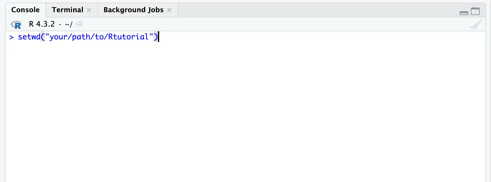
- In Console area, type the code as shown in the image below:
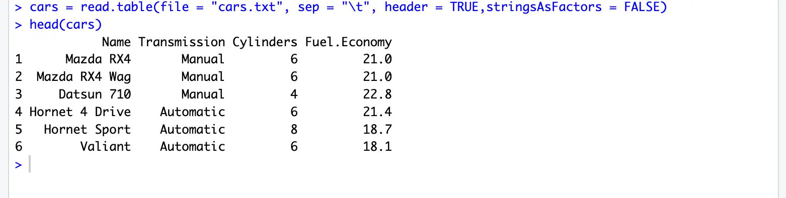
cars = read.table(file = "cars.txt", sep = "\t", header = TRUE,stringsAsFactors = FALSE)file: filename to read, e.g. cars.txt
header: logical (TRUE/ FALSE). TRUE means the first line contains the header or name of the variables, e.g. ‘mgp’,‘cyl’, ‘disp’
sep: data separator, "\t" means data is separated by tab. It can be whitespace, comma, newline or carriage returns.
To see the other parameters, type ?read.table() for further details.
cars <- read.table("cars.txt", header = T, sep = "\t")
nrow(cars) # get the number of rows
ncol(cars) # get the number of columns
head(cars) # preview the data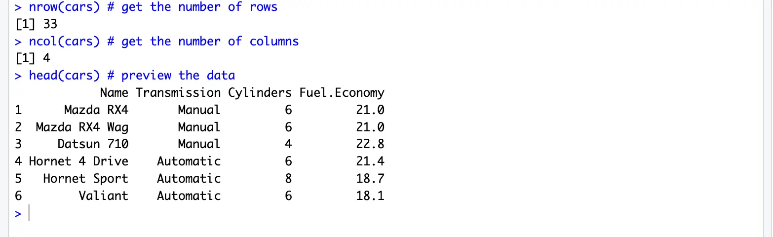
read.table() documentation: https://www.rdocumentation.org/packages/utils/versions/3.6.2/topics/read.table
cars[1, ] # extract the first row
cars[1:3, ] # extract the first 3 rows
cars[,"Transmission"] # extract the column named Cylinders
cars[ ,1] # extract the first column
cars[2,3] # extract the element at row 2 and column 3
cars[2:6, 2:4] # extract the elements at that range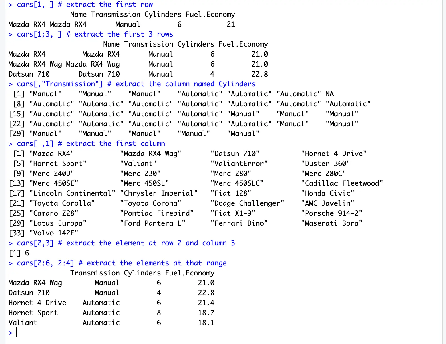
write.table(x, file, row.names, col.names, quote, sep )x: data you want to write on a file
file: name of the file on which you want to write
row.names / col.names: can be logical (TRUE/FALSE) or you can give values
quote: logical (TRUE/FALSE) whether you want to add quotes on your data frame
sep: how do you want to separate the data. Can be space or "\t" (tab)
write.table(x = cars,file = "modified_cars.txt",row.names = FALSE,sep= "\t")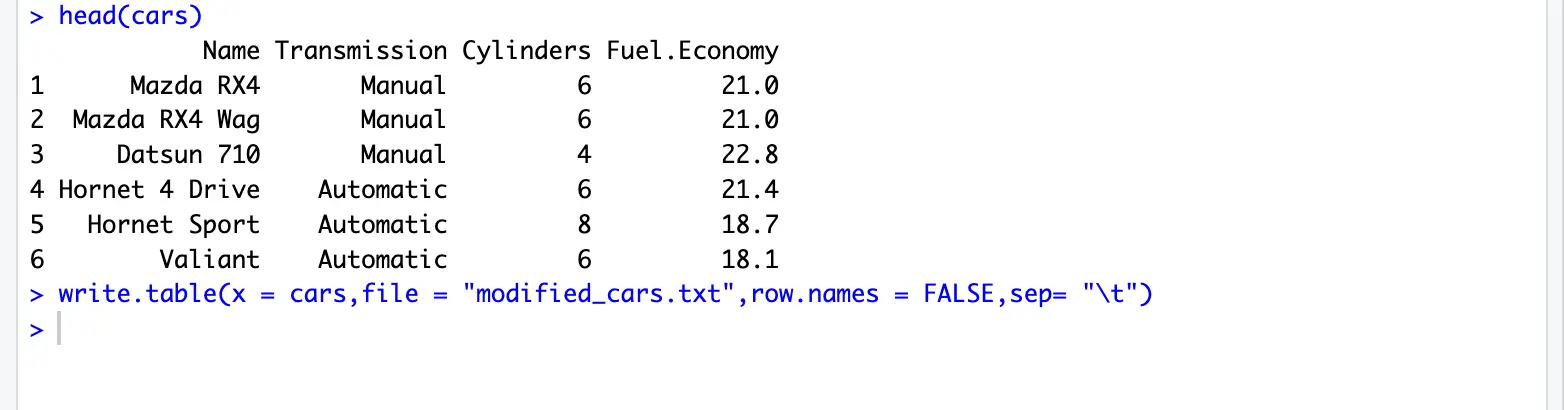
A csv file can be read in the following two ways:
data <- read.table("filename.csv", header = T, sep = ",")Note: we only changed name of the file from .txt to .csv and sep is changed to ",".
data <- read.csv("filename.csv", header = T)All the read.table() parameters are also applicable for read.csv().
Data can be saved as a csv file in the following two ways:
write.table(x = data, file = "filename.csv", sep = ",") write.csv(x = data, file = "filename.csv")All the write.table() parameters are also applicable for write.csv().
R provides its own format for saving or loading the data or R objects.
The two formats are RData or RDS.
These formats are useful in compressing the data and uses less space on computer disk.
You can save one or more r objects or variables as RData.
# save(data you want to save, file = "name of the file.RData")
head(cars)
x = 1:10
x
save(list = c("cars","x"),file = "cars.RDdat")
# or
save(cars,x,file = "cars.RDdat")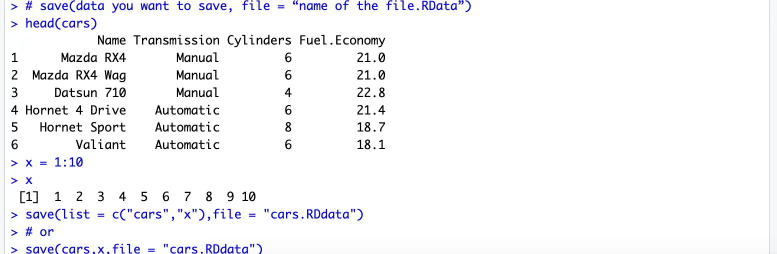
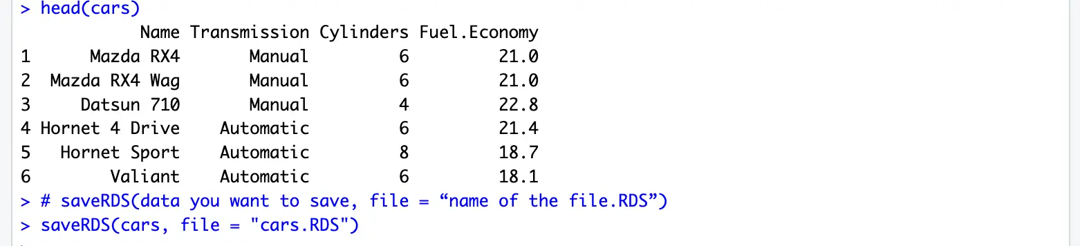
You can save only one r object or a variable in RDS format.
# saveRDS(data you want to save, file = "name of the file.RDS")
saveRDS(cars, file = "cars.RDS")
Note: You can use
compress = FALSEas a parameter in the save function to not compress the file.
# load(file = "filename to load.RData")
load(file = "cars.RDdata")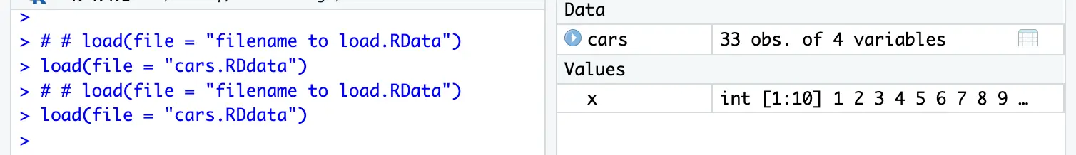
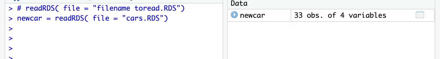
# readRDS( file = "filename to read.RDS")
newcar = readRDS( file = "cars.RDS")
You can assign a new name to the RDS data.
A package stores functions of a certain domain. For example, stats package contains functions in statistics.
Many functions are stored in standard packages which are delivered with R. But when you work with a particular domain (DNA microarray, for instance), usually you need to install outside packages.
Example: install a package named ggplot2. ggplot2 is an R package for producing statistical, or data, graphics. Unlike most other graphics packages, ggplot2 has an underlying grammar, based on the Grammar of Graphics, that allows you to compose graphs by combining independent components.
You can install ggplot2 R package by running:
install.packages("ggplot2")
# then following the download and install instructions.
Every time you run R/RStudio, it only loads standard packages. In order to use other installed packages, we need to load them.
library("ggplot2")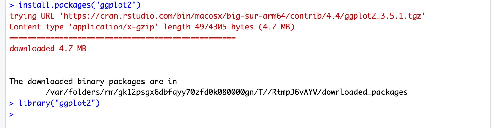
Setup steps: create a vector of random numbers:
# Load the required library
library(ggplot2)

# Generate two vectors 'x' and 'y' with 10 random numbers each, in the range [5, 6]
x <- runif(10, min = 5, max = 6)
y <- runif(10, min = 5, max = 6)

# Combine the vectors into a data frame for easier handling with ggplot2
data <- data.frame(x = x, y = y)

# Display the generated data
print(data)

# Create a scatter plot using ggplot2
ggplot(data, aes(x = x, y = y)) +
  geom_point()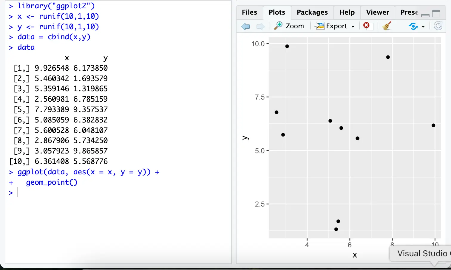
The plot will display in R's default plotting window. In RStudio, the plot will appear in the Plots pane (typically in the lower-right corner). You can export it as an image or PDF using the "Export" button.
For further information about ggplot2 R package, see: https://ggplot2-book.org
We use conditional statements when we want to execute some commands only when certain conditions are met.
Use if-statement to make a decision and execute different parts of the program based on the condition.
if (condition) {
# execute this part if condition holds true
}
All the commands you want to execute should be written here within curly braces
Example:
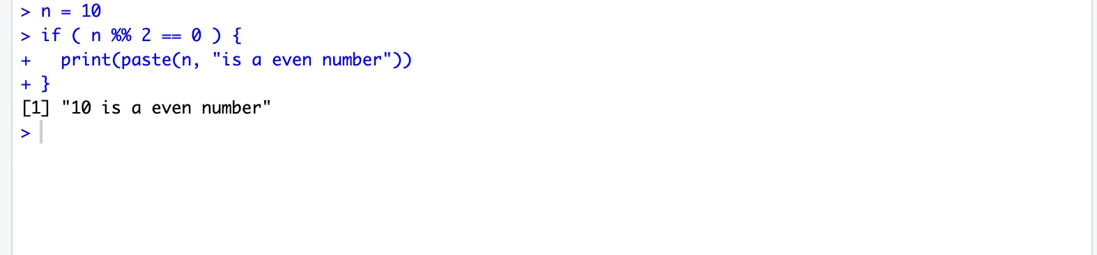
n = 10
if ( n %% 2 == 0 ) {
  print(paste(n, "is a even number"))
}
%% is the modulo operator and calculates the remainder. The line if(n %% 2==0) in essence means "Is the remainder of n divided by 2 equals to 0 ?", If n=10, then yes, it is. If n=11, or any odd number for that matter, then the remainder is not 0 and thus does not meet the condition.
ex: of conditions:
x <- 20
x > 10
x == 10
x %%10 ==2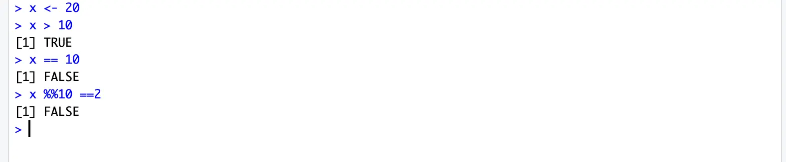
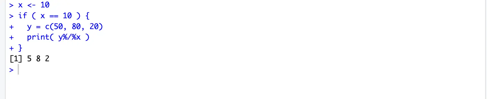
Use conditions like above in if statement ex:
x <- 10
if ( x == 10 ) {
  y = c(50, 80, 20)
  print( y%/%x )
}
We saw examples where condition is true, suppose we also want to execute different commands when the condition is false.
For that we add an else statement.
if (condition) {
# execute this part if condition holds true
}else {
# execute this part if condition is false
}
Example:
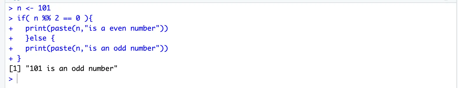
n <- 101
if( n %% 2 == 0 ){
  print(paste(n,"is a even number"))
  }else {
  print(paste(n,"is an odd number"))
}
if (condition_1) { # 1-1
  if (condition_2) { # 2-1
  # executes this part when both condition_1 and condition_2 are
  # true
  } # 2-2
  else { #3-1
  # executes this part when condition_1 is true but condition_2 is
  # false
  } # 3-2
} # 1-2
Curly braces are important here, they defines the scope of the statement for Example, curly braces 1-1 & 1-2 is the opening and closing of the first if statement which means, both if else are part of it and executed only when the first if is true.
Another way:
if (condition_1) { # 1-1
# condition_1
} # 1-2
else { # 2-1
if (condition_2) { # 3-1
# condition_2
} # 3-2
} # 2-2
You can directly use 'else if (condition)':
if (condition_1) {
# condition_1
} else if (condition_2) {
# condition_2
} else{
# condition_2
}
Example:
The letter grades of a class are evaluated based on the numeric grades:
| Numeric grade | Letter grade |
|---|---|
| 90-100 | A |
| 80-89 | B |
| 70-79 | C |
| 60-69 | D |
| < 60 | F |
numericGrade<- 80

if (numericGrade>=90) {
  letterGrade<-"A"
  } else if(numericGrade>=80){
    letterGrade<-"B"
    }else if(numericGrade>=70){
      letterGrade<-"C"
      }else if(numericGrade>=60){
        letterGrade<-"D"
        }else{
          letterGrade<-"F"
}

letterGrade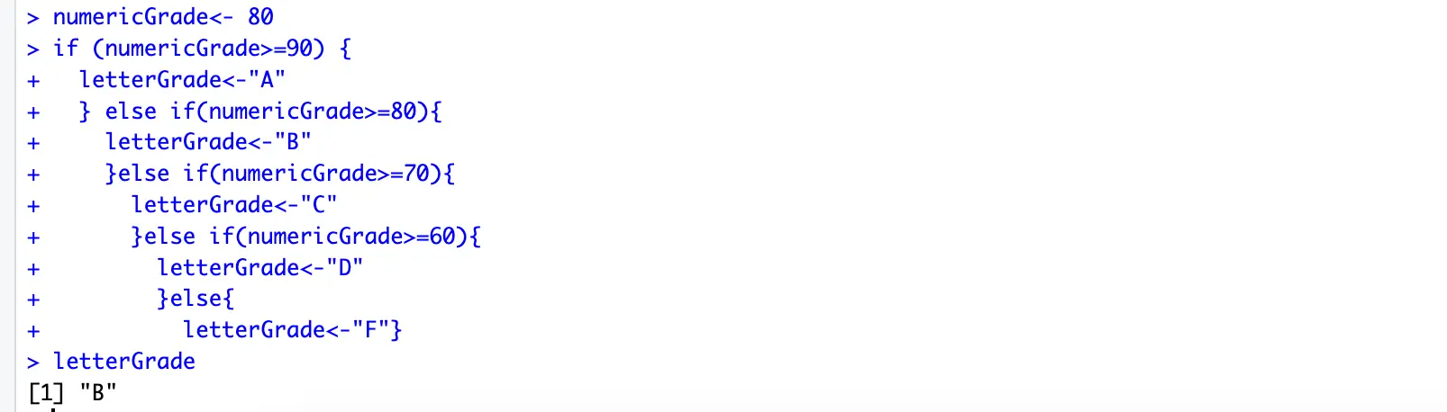
A loop is a mechanism to repeat a group of statements many times. Two most popular kind of loops are while-loop and for-loop
while (condition) {
# do something
}
The code inside the while-loop will be executed repeatedly until the condition becomes false. If the condition never gets to be false, then the loop is called infinite loop and the program runs forever. This situation must be avoided.
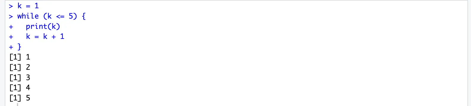
Example: Print numbers 1:5 using while loop.
- How many times loop should be iterated, here 5 times.
- Initialize a variable with 1, the name could be k or anything.
- Type "while" with parenthesis.
- Inside the parenthesis type your condition, since we do not want to go over 5, our condition would be k<=5.
- Write commands in the curly braces, here we want to print k.
- Do not forget to increment k, if you forget to increment k, your loop would not end as k is 1 every time and condition would be True every time.
R Code:
k = 1
while (k <= 5)
{
  print(k)
  k = k + 1
}
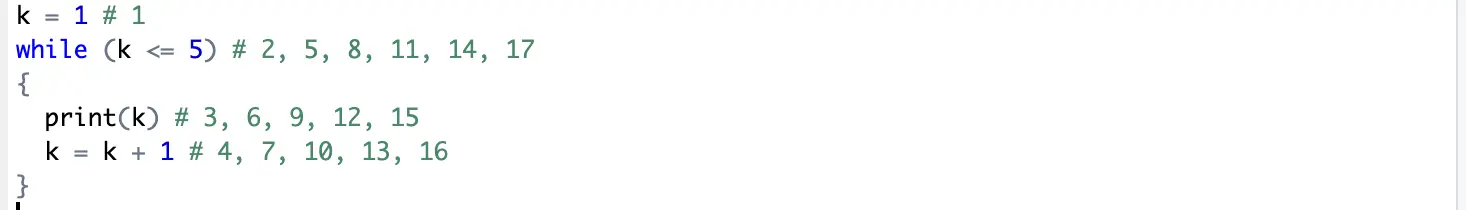
Control flow of the while loop example:
k = 1 # 1
while (k <= 5) # 2, 5, 8, 11, 14, 17
{
  print(k) # 3, 6, 9, 12, 15
  k = k + 1 # 4, 7, 10, 13, 16
}
| Step No. | k | operation |
|---|---|---|
| 1 | 1 | |
| 2 | 1 | While condition : TRUE |
| 3 | 1 | Print(k): 1 |
| 4 | 2 | k = k+1 |
| 5 | 2 | While condition: TRUE |
| 6 | 2 | Print(k): 2 |
| 7 | 3 | k = k + 1 |
| 8 | 3 | While condition: TRUE |
| 9 | 3 | Print(k): 3 |
| 10 | 4 | k = k + 1 |
| ... | ||
| ... | ||
| 17 | 6 | While condition: FALSE |
| Exit from the loop |
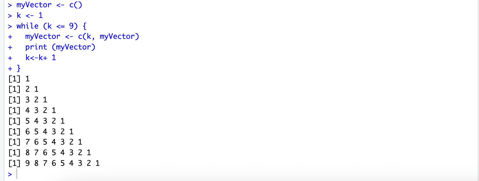
myVector <- c()
k <- 1
while (k <= 9) {
  myVector <- c(k, myVector)
  print (myVector)
  k<-k+ 1
}
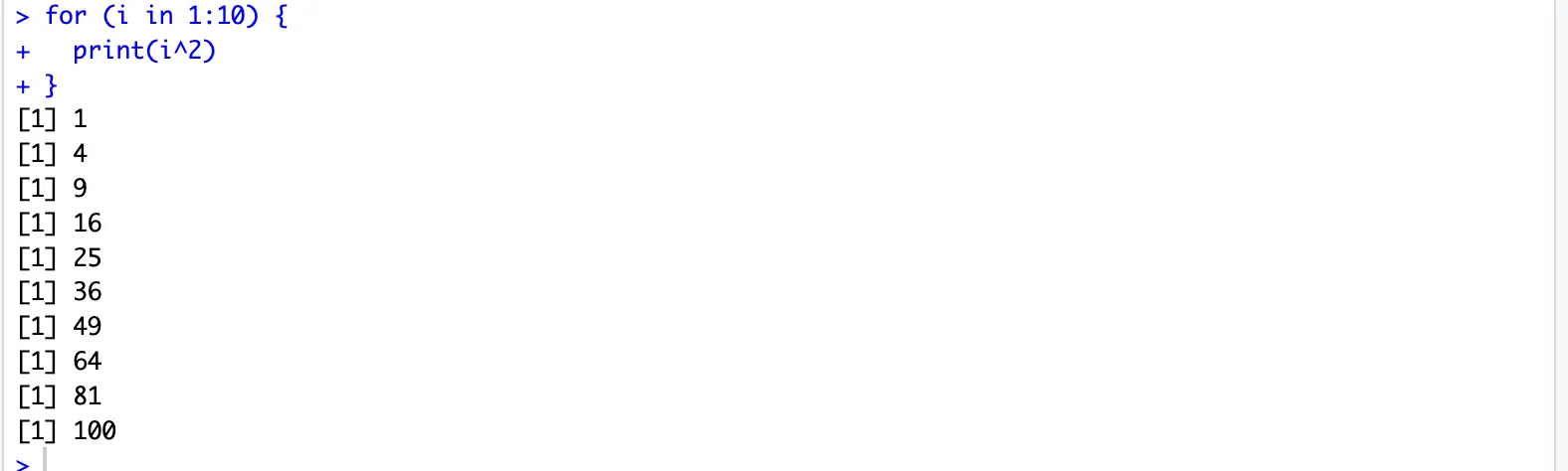
for-loop is more appropriate in situations of counting or indexing.
for (i in aVector) {
# do something
}
At every iteration, i is set to the value of an element from aVector.
Examples:
for (i in 1:10) {
  print(i^2)
}
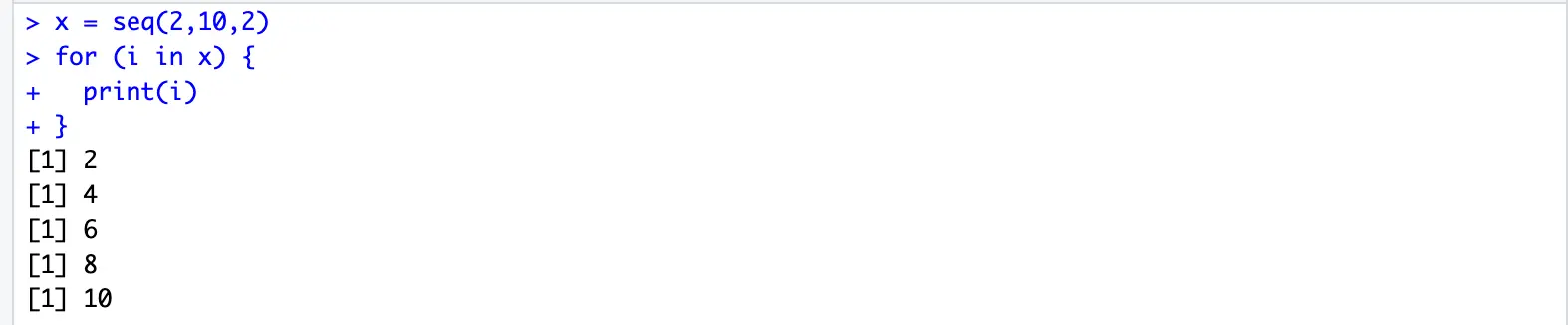
x = seq(2,10,2)
for (i in x) {
  print(i)
}
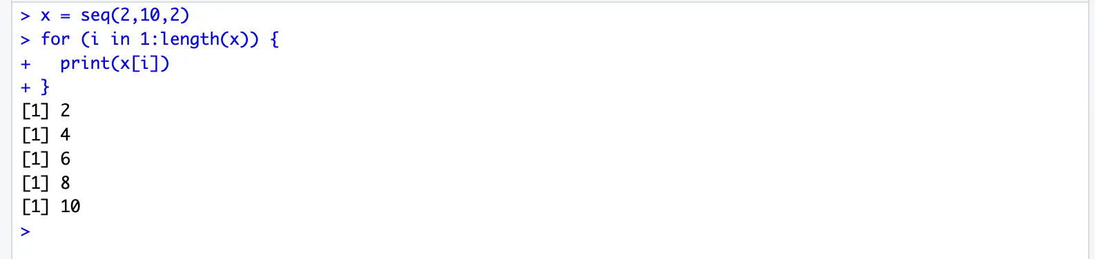
x = seq(2,10,2)
for (i in 1:length(x)) {
  print(x[i])
}
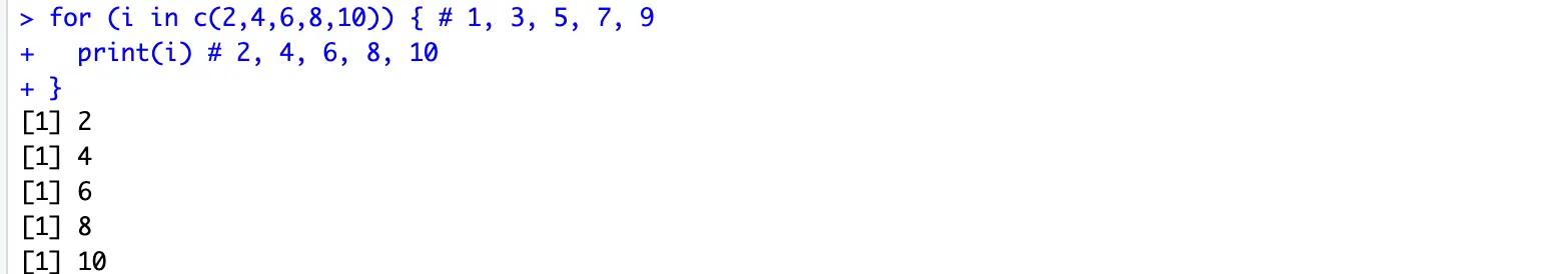
for (i in c(2,4,6,8,10)) { # 1, 3, 5, 7, 9
  print(i) # 2, 4, 6, 8, 10
}
Note: The green numbers in the example is the order by which code would be executed. At every iteration, i start from the value 2 and changes to 4, 6 ,8 and 10. The loop would end after i has been changed to last element.
| Step No. | k | operation |
|---|---|---|
| 1 | 2 | |
| 2 | 2 | Print(i) : 2 |
| 3 | 4 | |
| 4 | 4 | Print(i) : 4 |
| 5 | 6 | |
| 6 | 6 | Print(i): 6 |
| 7 | 8 | |
| 8 | 8 | Print(i) : 8 |
| 9 | 10 | |
| 10 | 10 | Print(i) : 10 |
| Exit from the loop |
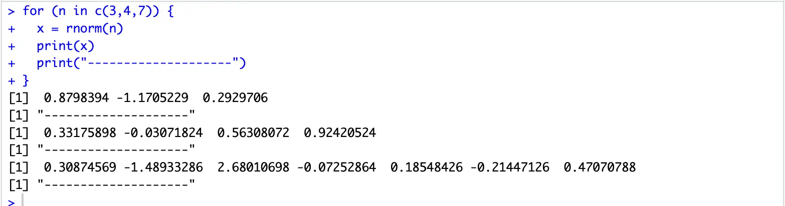
More examples:
for (n in c(3,4,7)) {
  x = rnorm(n)
  print(x)
  print("--------------------")
}
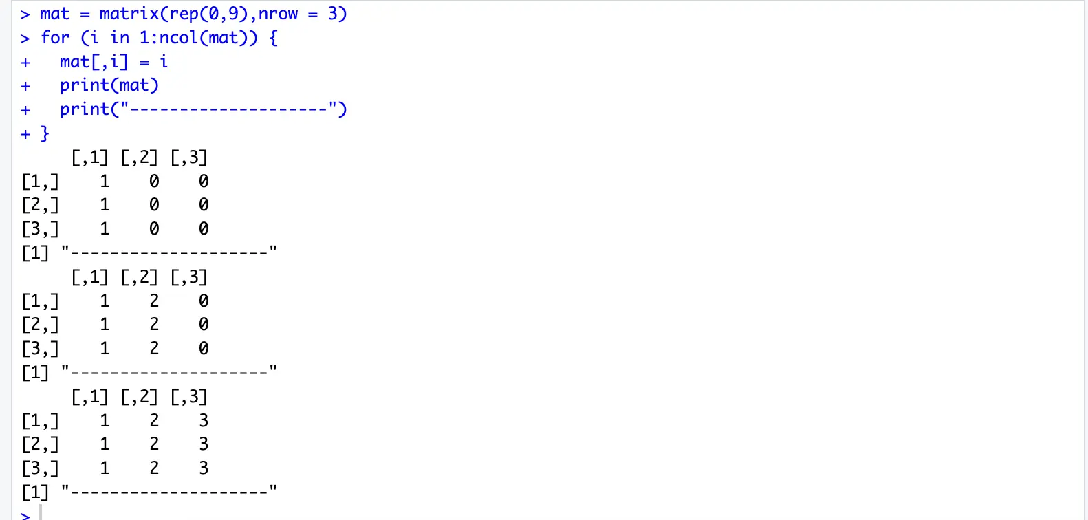
mat = matrix(rep(0,9),nrow = 3)
for (i in 1:ncol(mat)) {
  mat[,i] = i
  print(mat)
  print("--------------------")
}
In R, an implicit loop refers to performing operations on entire data structures (vectors, matrices, lists, etc.) without writing explicit for or while loops. Instead of looping over elements manually, you apply a function or operation that works on the whole object at once.
Examples include:
-
Vectorized arithmetic: x + y (adds corresponding elements of x and y)
-
The apply() family (apply(), lapply(), sapply(), tapply())
-
Functions like colSums(), rowMeans(), etc.
| Feature | R | Python (without NumPy) | C / Java |
|---|---|---|---|
| Default data structure | Vectorized | Scalar or list | Scalar or array |
| Looping style | Implicit, vectorized | Explicit or use NumPy | Explicit loops |
| Example addition | x + y |
for i in range(len(x)): x[i] + y[i] |
for (int i = 0; i < n; i++) { ... } |
-
In R, operations apply automatically over entire vectors or matrices.
-
In Python, you'd need for loops or NumPy arrays for similar efficiency.
-
In languages like C or Java, you'd have to write explicit loops.
Using implicit loops in R is a powerful feature that enhances the efficiency and readability of your code. Here are some key reasons why implicit loops are preferred in R:
-
Performance — Implicit loops are written in C under the hood and are much faster than explicit for loops in R.
-
Cleaner code — Operations on entire datasets can often be written in one line, improving readability.
-
Fewer errors — No need to manage loop counters or indices manually.
-
R’s design philosophy — R was built for statistical computing and works best when you think in terms of operations on whole datasets rather than individual elements.
R provides a mechanism called implicit loop, which does the same thing as for- and while- loop, but more convenient and effective in R data structures(data frame, list, …).
Implicit loop: family of apply() function: sapply(), lapply(), apply() , tapply(), …, meaning a function is applied to the data.
Applying a function to margins of an array or matrix.
Syntax: apply(X, MARGIN,FUN)
-
X: input data, name of the array or matrix.
-
MARGIN:
1 : indicates rows, manipulation is performed on rows.
2 : indicates columns, manipulation is performed on columns.
c(1,2) : indicates rows and columns.
-
FUN : can be built in functions, like mean, sum , median or you can add your own function.
Gives output in the form of vector, list or array.
Given a matrix mtx as follows (note: byrow = TRUE fills the matrix row-wise, so each row is filled before moving to the next):
mtx = matrix(c(1,2,3,
               4,5,6,
               7,8,9), nrow = 3,byrow = TRUE)
mtx
Output:
     [,1] [,2] [,3]
[1,]    1    2    3
[2,]    4    5    6
[3,]    7    8    9
Extract the min value of each row:
apply(mtx, 1, min)Output:
[1] 1 4 7The second argument is set to 1 to specify that the function is applied to rows. If it’s set to 2, then the function will be applied to columns.
Extract the sum of each column:
apply(mtx, 2, sum)Output:
[1] 12 15 18The second argument is set to 2 to specify that the function is applied to columns. (This is equivalent to the colSums() function.)
You can create your own function.
The code below is returning the squared row elements of matrix mtx.
apply(mtx, 1, function(x) x^2)Output:
     [,1] [,2] [,3]
[1,]    1    4    9
[2,]   16   25   36
[3,] 49 64 81sapply(): s stands for simplified.
It takes vector, list or data frame as input.
Gives vector, list or data frame as output.
Syntax: sapply(X, FUN)
- X: input data, name of the vector, list or data.frame.
- FUN: can be built in functions, like mean, sum, median or you can add your own function.
# create a list
my_list <- list(1:10)
# apply a function to each element of the list
result <- sapply(my_list, function(x) x^2)
print(result)
# Output:
[1] 1 4 9 16 25 36 49 64 81 100The variable i runs from 1 to 10, each time its value is squared. Input: vector 1:10 Output: vector (1:10)^2
Compute S = 1 + 1/2 + 1/3 +.. + 1/100
s = sapply(1:100, function(i) 1/i)
sum(s)
# Output:
[1] 5.187378Given a list x as follows:
x <- list(1:2, 3:5)
x
# Output:
[[1]]
[1] 1 2
[[2]]
[1] 3 4 5Extract the first number of each element in the list.
sapply(x, function(i) i[1])[1] 1 3
A data.frame can also be given as input. Add 5 to each element of data.frame.
df <- data.frame(a = 1:2, b = 3:4, c = 5:6, d = 7:8)
df
# Output:
a b c d
1 1 3 5 7
2 2 4 6 8sapply(df, function(i){
i+5
})# Output:
a b c d
[1,] 6 8 10 12
[2,] 7 9 11 13Given a data frame order as follows:
  subtotal  salestax  shipping
1 29.67     2.24      4.25
2 26.49     2.00      1.35
3 42.61     3.22      1.00
4 26.35     1.99      2.12
5 46.06     3.48      4.23
Compute the total amount for each order (add all columns row wise):
order <- data.frame(subtotal = c(29.67, 26.49, 42.61, 26.35, 46.06),
                    salestax = c(2.24, 2.00, 3.22, 1.99, 3.48),
                    shipping = c(4.25, 1.35, 1.00, 2.12, 4.23))
sapply(1:nrow(order), function(i) {
  sum(order[i, ])
})
# Output:
[1] 36.16 29.84 46.83 30.46 53.77
lapply: Applies a function over a vector or a list. It always return elements in the form of list. sapply and lapply are almost the same, except that sapply can return a vector, dataframe or list, whereas lapply only returns a list.
Syntax: lapply(X, FUN)
-
X: input data, name of the vector, list or data.frame.
-
FUN: can be built in functions, like mean, sum , median or you can add your own function.
# create a list
my_list <- list(a = 1:5, b = 6:10, c = 11:15)
# apply a function to each element of the list
result <- lapply(my_list, function(x) x^2)
print(result)
# Output:
$a
[1] 1 4 9 16 25
$b
[1] 36 49 64 81 100
$c
[1] 121 144 169 196 225
The variable x runs through each element of the list, squaring each element.
Compute the total amount for each order (add all columns row wise):
order <- data.frame(subtotal = c(29.67, 26.49, 42.61, 26.35, 46.06),
                    salestax = c(2.24, 2.00, 3.22, 1.99, 3.48),
                    shipping = c(4.25, 1.35, 1.00, 2.12, 4.23))
lapply(1:nrow(order), function(i) {
  sum(order[i, ])
})
# Output:
[[1]]
[1] 36.16
[[2]]
[1] 29.84
[[3]]
[1] 46.83
[[4]]
[1] 30.46
[[5]]
[1] 53.77
lapply(order,sum) # Output:
$subtotal
[1] 171.18
$salestax
[1] 12.93
$shipping
[1] 12.95
tapply: Applies a function over subsets of a vector. It is used to apply a function to each subset of a vector, grouped by one or more factors.
Syntax: tapply(X, INDEX, FUN)
- X: a vector to which function is applied.
- INDEX: list of factors or groups of same length.
- FUN : can be built in functions, like mean, sum, median, or you can add your own function.
Given a data frame dat as follows:
    strategy     result
1   conservative 7.79
2   conservative 32.50
3   conservative 18.16
4   conservative 56.87
5   aggressive   47.29
6   aggressive   49.38
7   aggressive   6.77
8   aggressive   44.43
9   moderate     51.68
10  moderate     25.05
11  moderate     29.54
12  moderate     56.30
Compute the average value for each strategy:
dat <- data.frame(strategy = c("conservative", "conservative",
                               "conservative","conservative",
                               "aggressive", "aggressive",
                               "aggressive", "aggressive",
                               "moderate","moderate",
                               "moderate", "moderate"),
                  result = c(7.79, 32.50,
                             18.16, 56.87,
                             47.29, 49.38,
                             6.77, 44.43,
                             51.68, 25.05,
                             29.54, 56.30))

tapply(dat$result, dat$strategy, mean)
# Output:
aggressive conservative moderate
36.9675 28.8300 40.6425
- First argument dat$result is the data.
- Second argument dat$strategy is the groups.
- Third argument mean is the function to apply.
- The output is the mean for each strategy.
Within practical experiments, sometimes the data cannot be collected. For instance, a mouse dies ahead of the measurement time, or a person quits in the middle of the experiment.
In those cases, empty data will be marked by NA (Not Applicable).
These NA slots affect most of the functions in R. Most of the time, you need to exclude those NAs before doing the computation.
For example:
x <- c(10, 20, NA, NA, 50)
mean(x)
sum(x)
# Output:
[1] NA
[1] NA
Note: sum() and mean() give NA results because some elements are NAs.
Find positions of NA elements
x <- c(10, 20, NA, NA, 50)
is.na(x)
which(is.na(x))
# Output:
[1] FALSE FALSE TRUE TRUE FALSE
[1] 3 4
Exclude NA from the vector
x <- c(10, 20, NA, NA, 50)
mean(x, na.rm = TRUE)
sum(x, na.rm = TRUE)
# Output:
[1] 26.66667
[1] 80
or
x <- c(10, 20, NA, NA, 50)
x[!is.na(x)]
mean(x[!is.na(x)])
sum(x[!is.na(x)])
# Output:
[1] 10 20 50
[1] 26.66667
[1] 80
x <- c(10, 20, NA, NA, 50)
sapply(x, function(i) i^2)
sapply(x, function(i) i^2, na.rm = TRUE)
sapply(x[!is.na(x)], function(i) i^2)
# Output:
[1] 100 400 NA NA 2500
[1] 100 400 2500
[1] 100 400 2500
On a data frame named order:
order <- data.frame(
  subtotal = c(49.92, 49.30, 38.20, 44.55, 42.33),
  salestax = c(3.77, 3.73, 2.89, 3.37, 3.20),
  shipping = c(2.67, NA, 4.91, NA, 3.62)
)
order
colSums(order)
# Output:
subtotal salestax shipping
1 49.92 3.77 2.67
2 49.30 3.73 NA
3 38.20 2.89 4.91
4 44.55 3.37 NA
5 42.33 3.20 3.62
[1] 224.30 16.96 NA
Some functions integrate NA removal into the parameter, na.rm means "remove NA".
apply(order, 2, mean)
apply(order, 2, mean, na.rm = TRUE)
# Output:
subtotal salestax shipping
44.860 3.392 NA
subtotal salestax shipping
44.860000 3.392000 3.733333
Further reading
apply https://www.youtube.com/watch?v=f0U74ZvLfQo
lapply and sapply lapply and sapply
tapply tapply
Generic function to plot: plot().
Generic arguments:
• type: plot type. p for points, l for lines, b for both points and lines, h for histogram-like vertical lines, s for stair steps, n for no plotting.
• main: title of the plot.
• xlab: label of x-axis.
• ylab: label of y-axis.
Example: plot the function y = sin(x):
x <- seq(0, 2 * pi, length.out = 100)
y <- sin(x)
plot(x, y)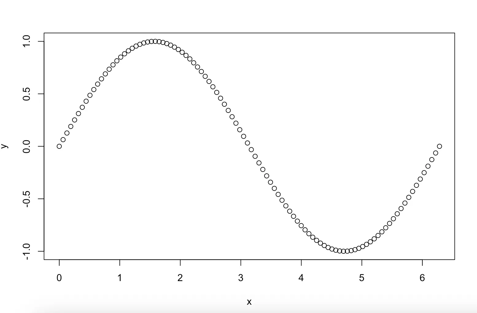
plot(x,y,type = "l", main = "Graph of sinus function")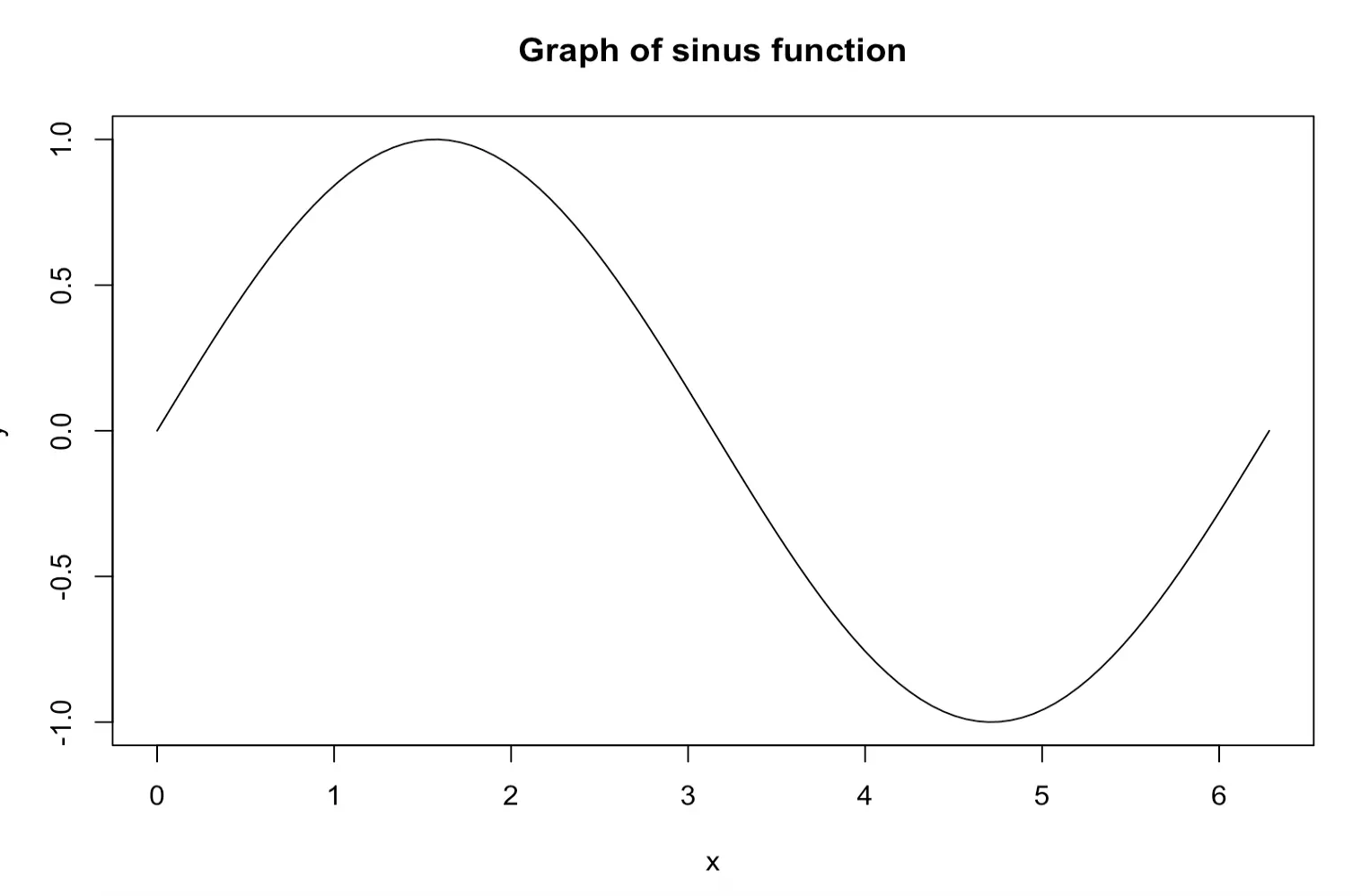
Remember to set working directory so that the files go to the right place. Save as bitmap file:
bmp("sinus.bmp") # open/create the file
plot(x,y,type = "l", main = "Graph of sinus function")
dev.off() # close the file
Save as jpeg file: just different at the command to open the file
jpeg("sinus.jpg") # open/create the file
plot(x,y,type = "l", main = "Graph of sinus function")
dev.off() # close the file
Save as png file:
png("sinus.png") # open/create the file
plot(x,y,type = "l", main = "Graph of sinus function")
dev.off() # close the file
Save as pdf file:
pdf("sinus.pdf") # open/create the file
plot(x,y,type = "l", main = "Graph of sinus function")
dev.off() # close the file
Or you can save the image directly from the plot window.
The plot of the next example is called scatter plot. Basically, it shows the relationship of two variables. And when you have data for two variables, scatter plot would be the first to consider.
Another example: cars data frame, which is built-in R:
data(cars)
head(cars)
plot(cars$speed, cars$dist, main = "Cars data", xlab = "Speed (mph)", ylab = "Distance (ft)", pch = 19, col = "blue")
speed dist
1 4 2
2 4 10
3 7 4
4 7 22
5 8 16
6 9 10
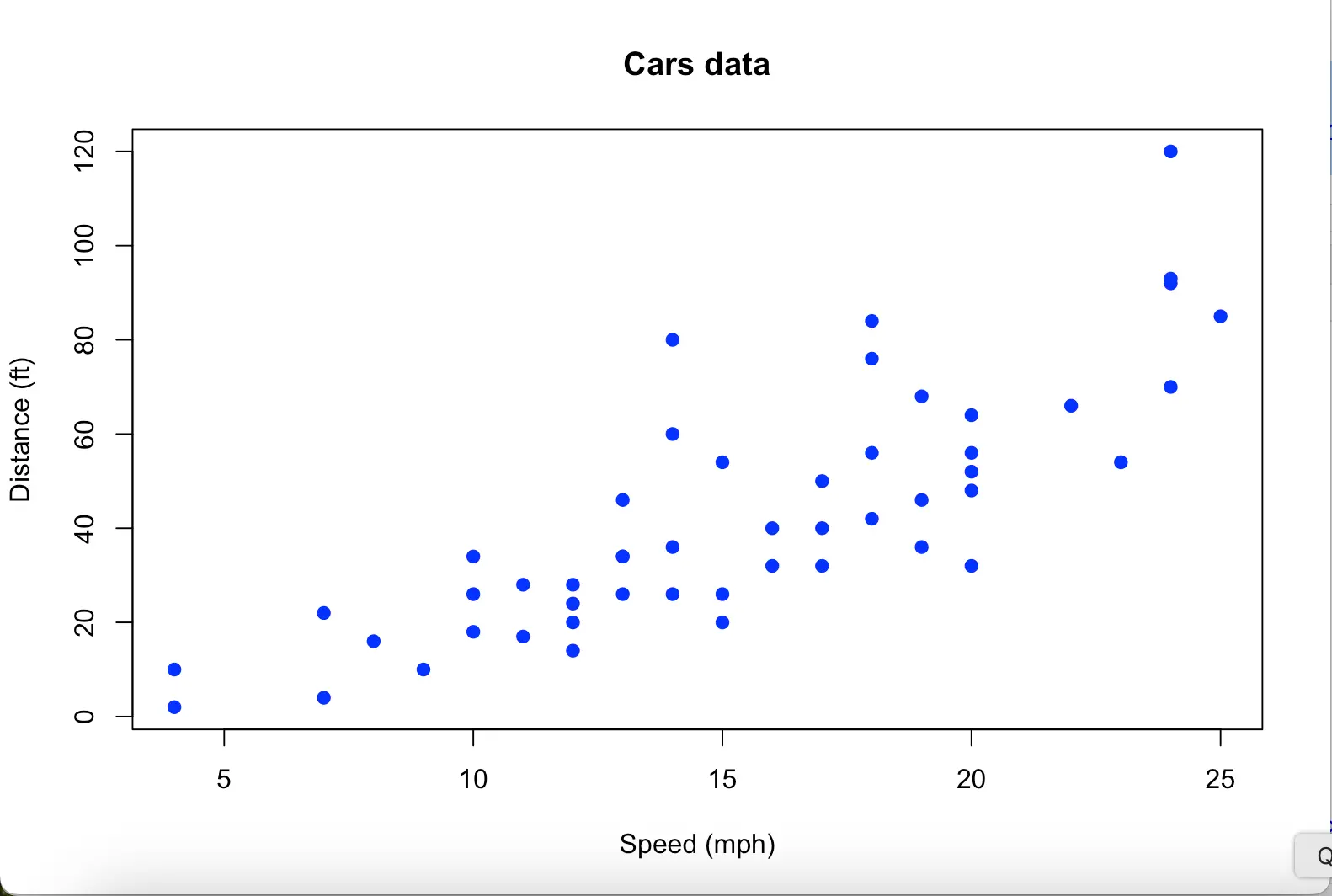
cars has two variables:
speed: miles per hour
dist: distance to stop (feet)
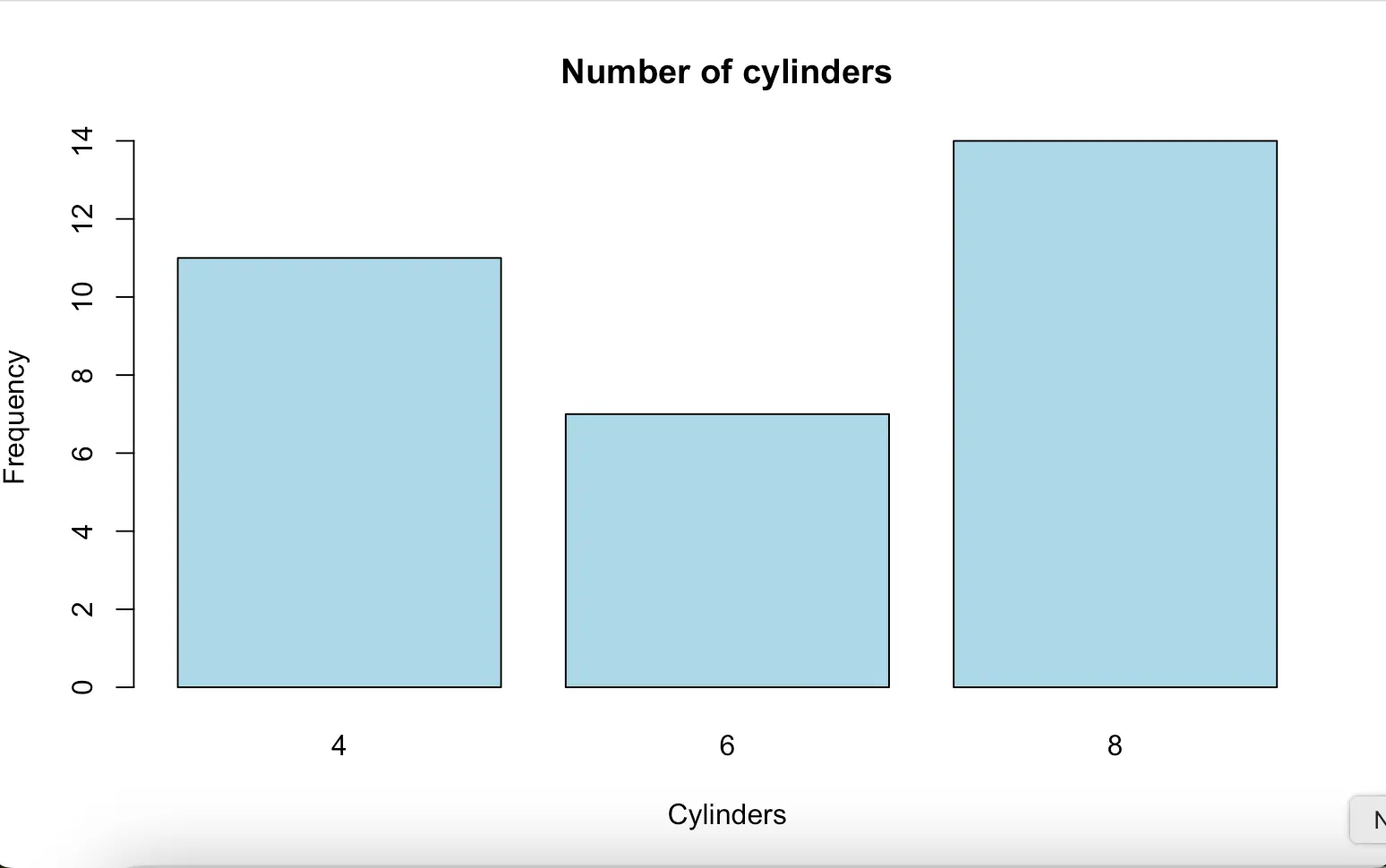
Bar plot is used to show the distribution of a categorical variable. Example: mtcars data frame, which is built-in R:
data(mtcars)
head(mtcars)
table(mtcars$cyl)
barplot(table(mtcars$cyl), main = "Number of cylinders", xlab = "Cylinders", ylab = "Frequency", col = "lightblue")
mpg cyl disp hp drat wt qsec vs am gear carb
Mazda RX4 21.0 6 160 110 3.90 2.620 16.46 0 1 4 4
Mazda RX4 Wag 21.0 6 160 110 3.90 2.875 17.02 0 1 4 4
Datsun 710 22.8 4 108 93 3.85 2.320 18.61 1 1 4 1
Hornet 4 Drive 21.4 6 258 110 3.08 3.215 19.44 1 0 3 1
Hornet Sportabout 18.7 8 360 175 3.15 3.440 17.02 0 0 3 2
Valiant 18.1 6 225 105 2.76 3.460 20.22 1 0 3 1
4 6 8
11 7 14
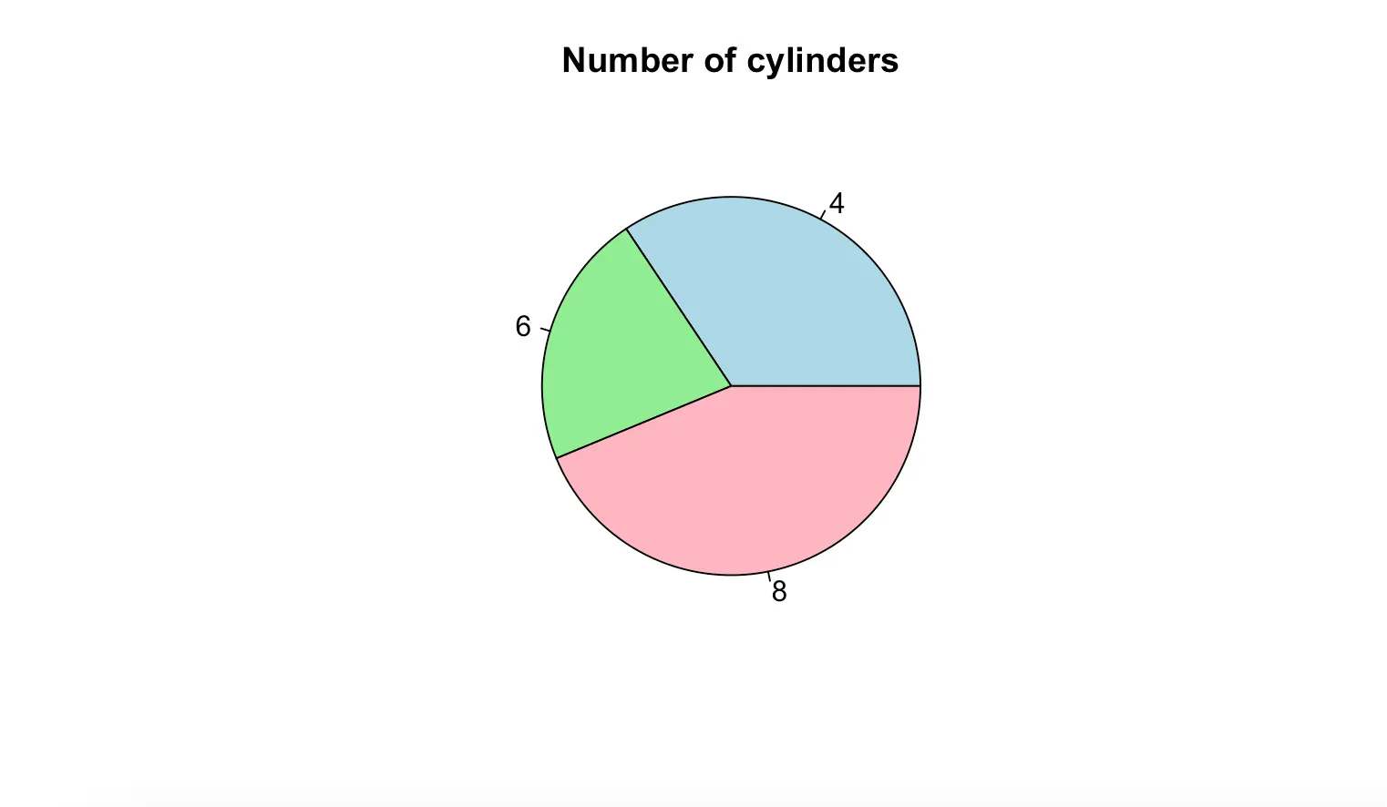
Pie plot is also used to show the distribution of a categorical variable. Example: mtcars data frame, which is built-in R:
data(mtcars)
table(mtcars$cyl)
pie(table(mtcars$cyl), main = "Number of cylinders", col = c("lightblue", "lightgreen", "lightpink"))
4 6 8
11 7 14
The labels variable is used to display the details that each slice represents in the pie chart.
pct <- round(table(mtcars$cyl)/sum(table(mtcars$cyl))*100)
pielabels <- paste(c("4 cyl", "6 cyl", "8 cyl"), "\n", pct, "%", sep = "")
pie(table(mtcars$cyl), main = "Number of cylinders", col = c("lightblue", "lightgreen", "lightpink"), labels = pielabels) 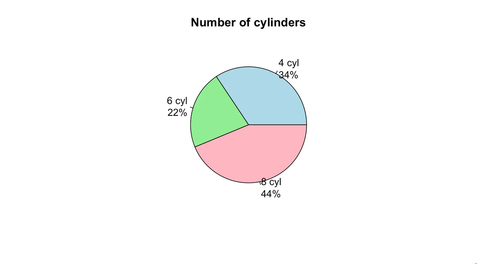
3D pie chart is more attractive than 2D pie chart.
Package needed: plotrix. Install it first if you do not have it.
library(plotrix)
pct <- round(table(mtcars$cyl)/sum(table(mtcars$cyl))*100 )
pielabels <- paste(c("4 cyl", "6 cyl", "8 cyl"), "\n", pct, "%", sep = "")
pie3D(table(mtcars$cyl), main = "Number of cylinders", col = c("lightblue", "lightgreen", "lightpink"), labels = pielabels, explode = 0.1)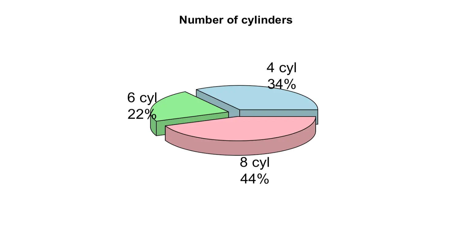
A histogram is a simple yet powerful tool to visualize the distribution of numeric data. It works by splitting the range of values into intervals (called bins) and counting how many data points fall into each interval. The counts are then displayed as bars.
Example Code:
# suppose our data are 100 random numbers created by rnorm()
x <- rnorm(100)
# plot the histogram
hist(x)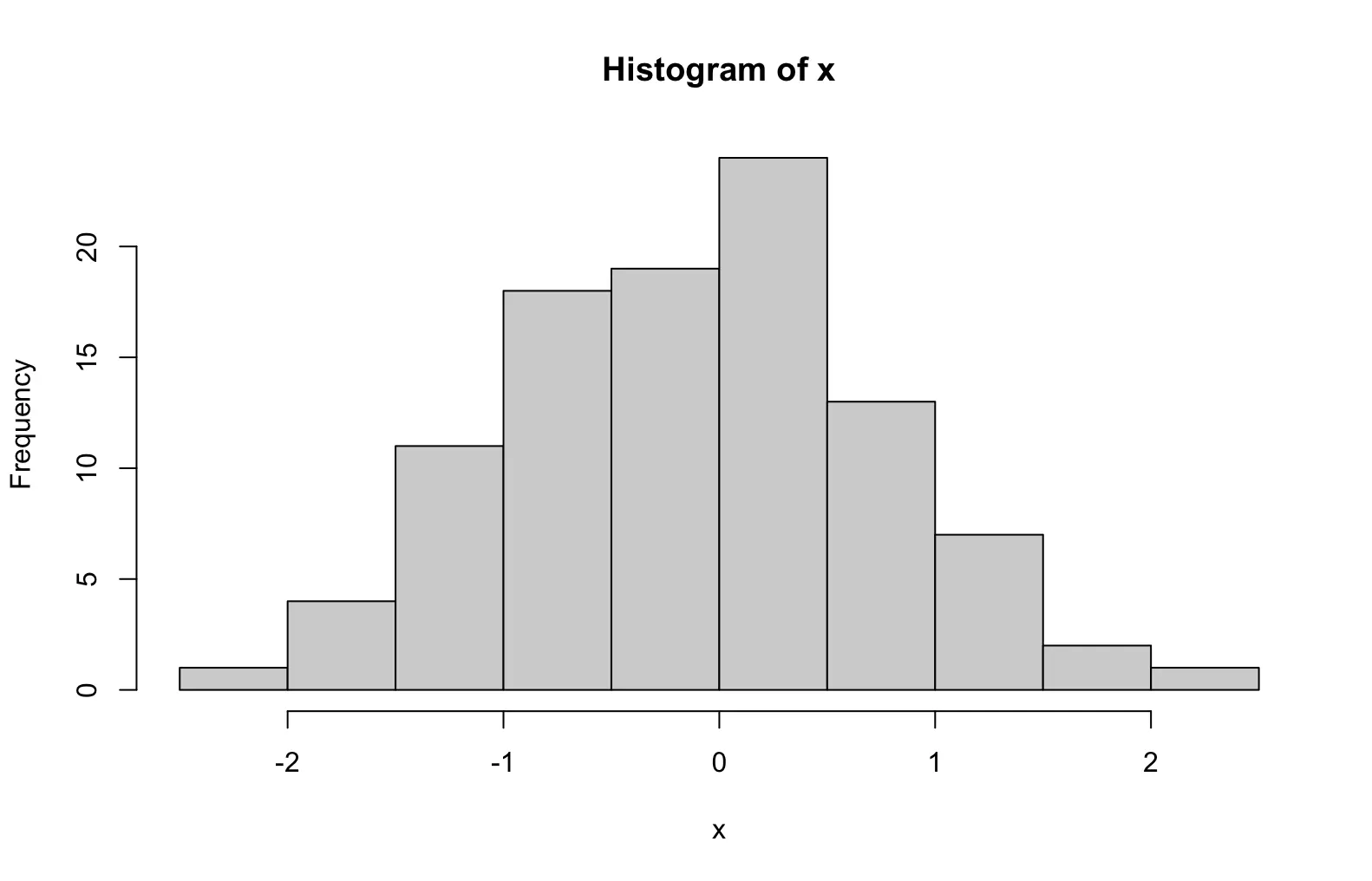
The histogram shows:
-
X-axis (horizontal) → the range of values.
-
Y-axis (vertical) → the frequency (number of observations) in each bin.
Since the data come from a normal distribution, the histogram typically looks like a “bell curve,” with most values around 0 and fewer values toward the extremes.
Customizing the Histogram:
The hist() function has several options to make your plots clearer and more informative:
hist(x,
     breaks = 20,                   # number of bins
     col = "lightblue",             # bar color
     border = "white",              # border color
     main = "Histogram of Normal Data", # title
     xlab = "Value",                # x-axis label
     ylab = "Frequency")            # y-axis label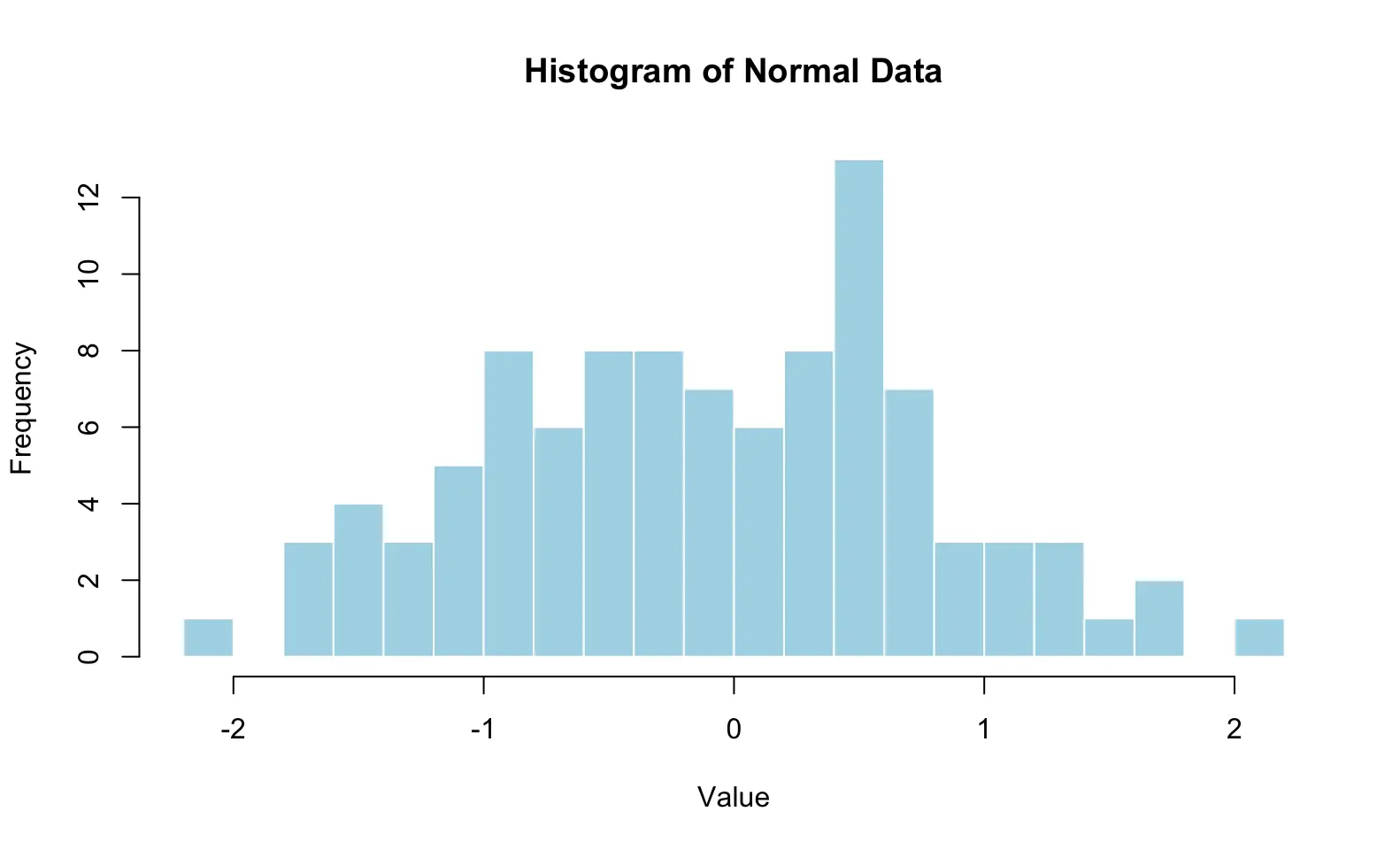
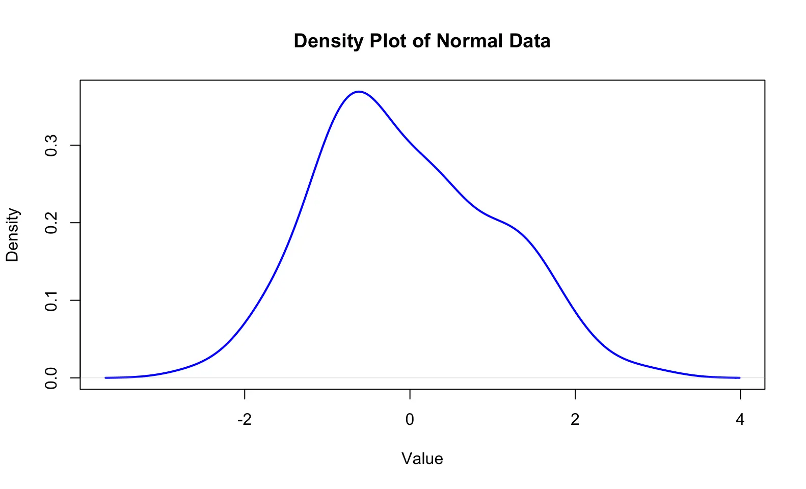
A density plot is a smoothed version of a histogram that estimates the probability density function of a continuous variable. It provides a continuous curve that represents the distribution of the data, making it easier to visualize the shape of the distribution. Example Code:
# suppose our data are 100 random numbers created by rnorm()
x <- rnorm(100)
# plot the density
plot(density(x),
     main = "Density Plot of Normal Data", # title
     xlab = "Value",                        # x-axis label
     ylab = "Density",                      # y-axis label
     col = "blue",                          # line color
     lwd = 2)                               # line width
Note that the vertical axis becomes %,not count numbers anymore.
A box plot (or box-and-whisker plot) is a graphical representation of the distribution of a dataset that highlights its central tendency, variability, and potential outliers. It provides a visual summary of key statistical measures, including the median, quartiles, and extremes. Example Code:
#Using the built-in data frame mtcars
data(mtcars)
# Create a box plot of miles per gallon (mpg) grouped by the number of cylinders
boxplot(mpg ~ cyl, data = mtcars,
        main = "Box Plot of MPG by Number of Cylinders", # title
        xlab = "Number of Cylinders",                     # x-axis label
        ylab = "Miles Per Gallon (MPG)",                 # y-axis label
        col = c("lightblue", "lightgreen", "lightpink")) # box colors
        # boxplot of mpg by cylinders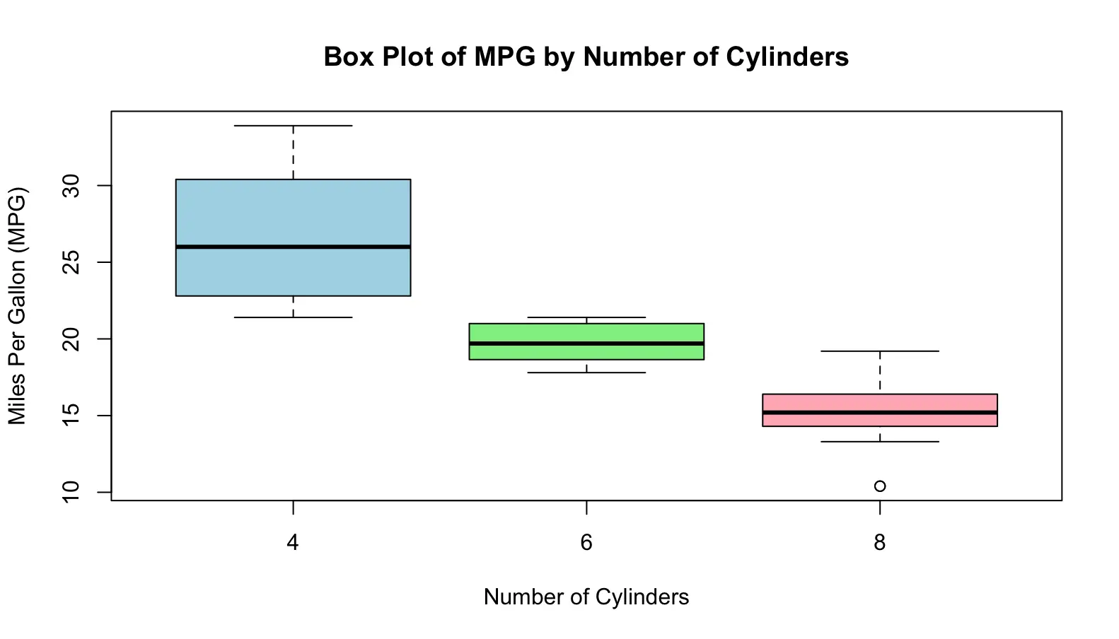
Individuals are objects described in the dataset. Individuals can be people, animals, or things.
A variable is a characteristic of an individual. A variable can take different values for different individuals.
| Name | Year | Gender | Grade |
|---|---|---|---|
| Luke | Sophomore | F | 95 |
| Jennifer | Freshman | M | 92 |
| Sam | Sophomore | M | 78 |
| Anna | Junior | F | 75 |
For example, in a class roster, each student is an individual. Name, Year, Gender, Grade are variables.
A categorical variable places an individual into one of several groups or categories.
A quantitative variable takes numerical values for which arithmetic operations such as adding and averaging make sense.
In the class roster example, Year and Gender are categorical variables; Grade is a quantitative variable
The distribution of a variable tells us what values it takes and how often it takes these values.
The values of a categorical variable are labels for the categories, for example Male and Female.
The distribution of a categorical variable lists the categories and gives either the count or the percent of individuals who fall in each category.
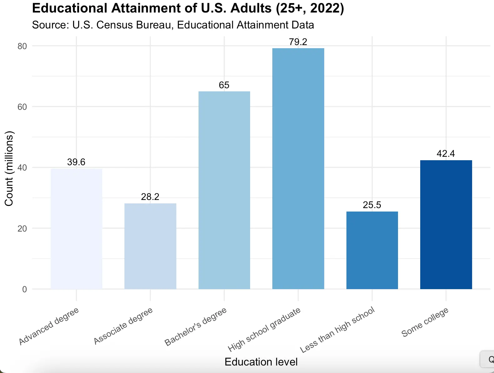
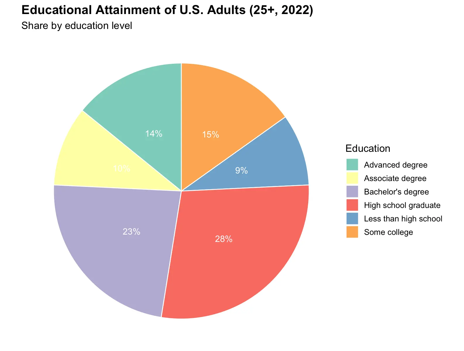
Example: distribution of the highest education level for people aged 25-34
| Education | Count (millions, approx.) | Percent (%) |
|---|---|---|
| Less than high school | 25.5 | 9.0 |
| High school graduate | 79.2 | 28.0 |
| Some college | 42.4 | 15.0 |
| Associate degree | 28.2 | 10.0 |
| Bachelor's degree | 65.0 | 23.0 |
| Advanced degree | 39.6 | 14.0 |
# Load ggplot2
library(ggplot2)

# Reference: https://www.census.gov/newsroom/press-releases/2023/educational-attainment-data.html
edu_data <- data.frame(
  Education = c("Less than high school",
                "High school graduate",
                "Some college",
                "Associate degree",
                "Bachelor's degree",
                "Advanced degree"),
  Count_millions = c(25.5, 79.2, 42.4, 28.2, 65.0, 39.6),
  Percent = c(9.0, 28.0, 15.0, 10.0, 23.0, 14.0)
)

# Bar plot with ggplot2
ggplot(edu_data, aes(x = Education, y = Count_millions, fill = Education)) +
  geom_col(width = 0.7, show.legend = FALSE) +
  geom_text(aes(label = Count_millions),
            vjust = -0.5, size = 4) +
  scale_fill_brewer(palette = "Blues") +
  labs(title = "Educational Attainment of U.S. Adults (25+, 2022)",
       subtitle = "Source: U.S. Census Bureau, Educational Attainment Data",
       x = "Education level",
       y = "Count (millions)") +
  theme_minimal(base_size = 13) +
  theme(axis.text.x = element_text(angle = 30, hjust = 1),
        plot.title = element_text(face = "bold", size = 16))

# Pie chart of Percent
ggplot(edu_data, aes(x = "", y = Percent, fill = Education)) +
  geom_col(width = 1, color = "white") +
  coord_polar(theta = "y") +
  geom_text(aes(label = paste0(Percent, "%")),
            position = position_stack(vjust = 0.5), size = 4, color = "white") +
  scale_fill_brewer(palette = "Set3") +
  labs(title = "Educational Attainment of U.S. Adults (25+, 2022)",
       subtitle = "Share by education level",
       fill = "Education") +
  theme_void(base_size = 13) +
  theme(plot.title = element_text(face = "bold", size = 16))
A histogram divides the range of a quantitative variable into intervals (called bins or classes) and displays the count or percentage of observations within each interval. To accurately represent the distribution, bins should be of equal width.
Example:
Exam scores: [70,80), [80,90), ..., [150,160]
The number of individuals in each bin is called the frequency.
set.seed(123)  # for reproducibility
scores <- round(rnorm(100, mean = 110, sd = 15))  # 100 exam scores, mean ~110

# Quick summary
summary(scores)

# Histogram
hist(scores,
  breaks = seq(70, 160, by = 10),  # bins: [70,80), [80,90), ..., [150,160]
  main = "Distribution of Exam Scores",
  xlab = "Score",
  ylab = "Frequency",
  col = "lightblue",
  border = "white")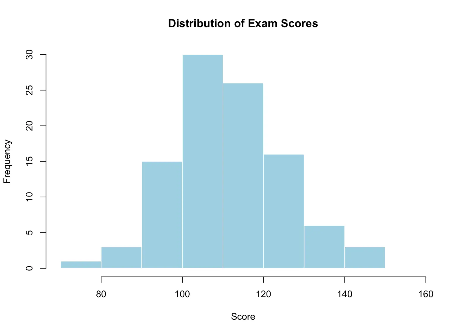
Histograms are useful for visualizing the shape, center, and spread of quantitative data, and for identifying outliers or unusual patterns.
When analyzing a graph of data, look for the overall pattern as well as any notable deviations from that pattern. You can describe the overall pattern of a distribution by considering its shape, center, and spread.
- Outliers: Values that fall outside the general pattern.
- Modes: Major peaks in the distribution. A distribution is called unimodal if it has one major peak (as in the Exam Score example).
- Symmetry: A distribution is symmetric if values below and above its midpoint are mirror images of each other (the Exam Score histogram is symmetric).
- Skewness: A distribution is skewed to the right if the right tail (larger values) is much longer than the left tail (smaller values).
Histogram with outliers:
set.seed(123)  # for reproducibility
scores_with_outliers <- c(round(rnorm(95, mean = 110, sd = 15)), 30, 45, 180, 200, 220)  # add some outliers
# Quick summary
summary(scores_with_outliers)
# Histogram
hist(scores_with_outliers,
     breaks = seq(20, 230, by = 10),  # bins: [20,30), [30,40), ..., [220,230)
     main = "Distribution of Exam Scores with Outliers",
     xlab = "Score",
     ylab = "Frequency",
     col = "lightcoral",
     border = "white")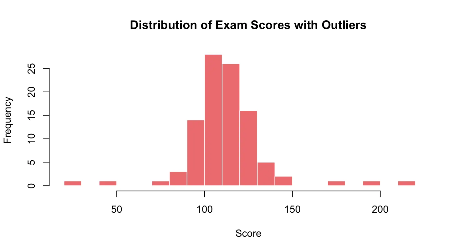
Right-skewed histogram:
set.seed(123)  # for reproducibility
scores_right_skewed <- c(round(rnorm(80, mean = 100, sd = 10)), round(rnorm(20, mean = 150, sd = 10)))  # right-skewed data
# Quick summary
summary(scores_right_skewed)
# Histogram
hist(scores_right_skewed,
     breaks = seq(60, 180, by = 10),  # bins: [60,70), [70,80), ..., [170,180)
     main = "Right-Skewed Distribution of Exam Scores",
     xlab = "Score",
     ylab = "Frequency",
     col = "lightgreen",
     border = "white")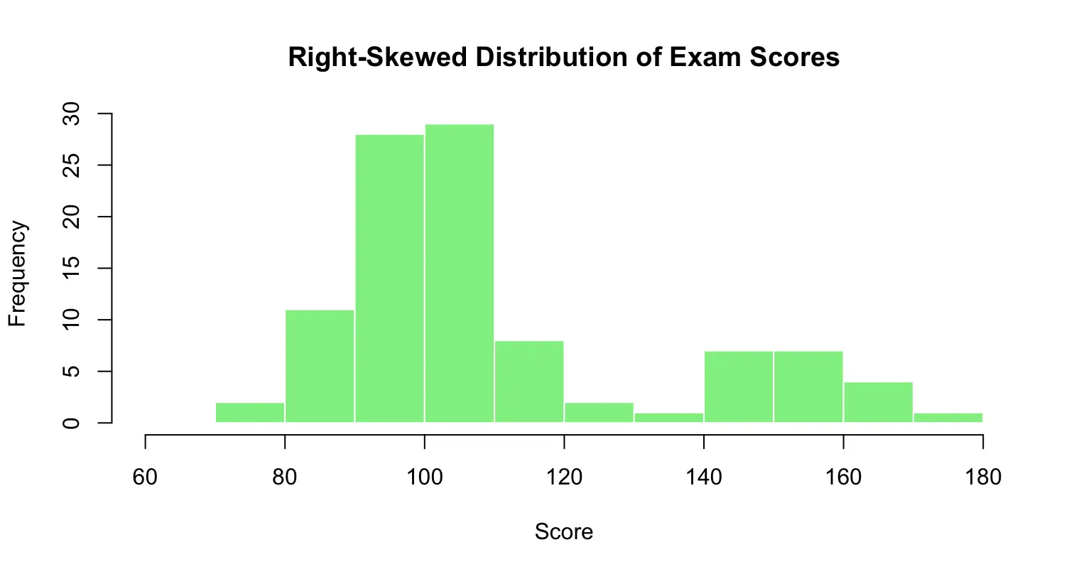
-
Mean: the average value
- If the
$n$ observations are$x_1, x_2, ..., x_n$ , their mean is:$\bar{x} = \frac{x_1 + x_2 + ... + x_n}{n}$
- If the
-
Median: the middle value
- Arrange all observations from smallest to largest.
- If
$n$ is odd, the median is the center observation in the ordered list. - If
$n$ is even, the median is the mean of the two center observations in the ordered list.
-
Mean vs. Median
- There are 100 people in a village. 99 people who are poor have to share 1 chicken. The one rich person has 99 chickens.
- Mean: each person has 1 chicken on average
$\rightarrow$ people are doing OK - Median: the middle person has 1/99 chicken
$\rightarrow$ people are hungry
Example: Exam scores
set.seed(123)
scores <- c(round(rnorm(95, mean = 110, sd = 15)), 300, 350, 400, 450, 500)  # 95 normal scores + 5 extreme outliers
mean_score <- mean(scores)
median_score <- median(scores)
mean_score
median_score
# Output:
[1] 125.64
[1] 112
-
Measure of center alone can be misleading.
- Two countries A and B have the same family income. (same mean/median)
- A has extremes of wealth and poverty. B has little variation among families.
-
$\rightarrow$ Both measure of center and measure of spread are needed.
-
Quartiles
$Q_1$ and$Q_3$ - Arrange all observations from smallest to largest and locate the median M.
- The first quartile
$Q_1$ is the median of those on the left of M. - The third quartile
$Q_3$ is the median of those on the right of M.
-
Examples
-
Sorted list: 19 22 23 23 23 25 26 27 28 29 29 31 32
-
Q1 = median(19 22 23 23 23 25) = 23
-
Q3 = median(27 28 29 29 31 32) = 29
-
Sorted list: 55 73 75 80 80 85 90 92 93 98
-
Q1 = median(55 73 75 80 80) = 75
-
Q3 = median(85 90 92 93 98) = 92
-
-
A descriptive statistics consists of 5 numbers from a set of observations:
- The min value
- The first quartile Q1
- The median
- The third quartile Q3
- The max value
-
In R, use
fivenum()function
> x <- c(19,22,23,23,23,25,26,27,28,29,29,31,32)
> fivenum(x)
[1] 19 23 26 29 32
> y <- c(55,73,75,80,80,85,90,92,93,98)
> fivenum(y)
[1] 55.0 75.0 82.5 92.0 98.0A boxplot (or box-and-whisker plot) is a graphical representation of the five-number summary of a dataset. It provides a visual summary of key statistical measures, including the minimum, first quartile (Q1), median, third quartile (Q3), and maximum. Boxplots are useful for comparing distributions across different groups or categories.
Minimum, Q1, Median (M), Q3, Maximum
A central box spans the quartiles Q1 and Q3, representing the interquartile range (IQR), which is calculated as
A line in the box marks the median M
Lines called "whiskers" extend from the box out to the smallest and largest observations that are not considered outliers; if there are outliers, the whiskers do not reach the absolute minimum or maximum.
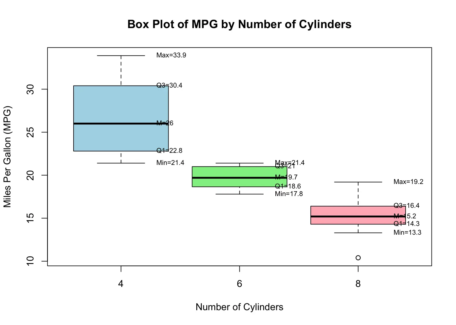
Example Code:
# Using the built-in data frame mtcars
data(mtcars)
# Create a box plot of miles per gallon (mpg) grouped by the number of cylinders
boxplot(mpg ~ cyl, data = mtcars,
        main = "Box Plot of MPG by Number of Cylinders", # title
        xlab = "Number of Cylinders",                     # x-axis label
        ylab = "Miles Per Gallon (MPG)",                 # y-axis label
        col = c("lightblue", "lightgreen", "lightpink")) # box colors
stats <- boxplot(mpg ~ cyl, data = mtcars, plot = FALSE)$stats

x_pos <- 1:ncol(stats)

for (i in x_pos) {
  text(x = i + 0.25, y = stats[1, i], labels = paste0("Min=", round(stats[1, i], 1)), pos = 4, cex = 0.7)
  text(x = i + 0.25, y = stats[2, i], labels = paste0("Q1=", round(stats[2, i], 1)), pos = 4, cex = 0.7)
  text(x = i + 0.25, y = stats[3, i], labels = paste0("M=", round(stats[3, i], 1)), pos = 4, cex = 0.7)
  text(x = i + 0.25, y = stats[4, i], labels = paste0("Q3=", round(stats[4, i], 1)), pos = 4, cex = 0.7)
  text(x = i + 0.25, y = stats[5, i], labels = paste0("Max=", round(stats[5, i], 1)), pos = 4, cex = 0.7)
}
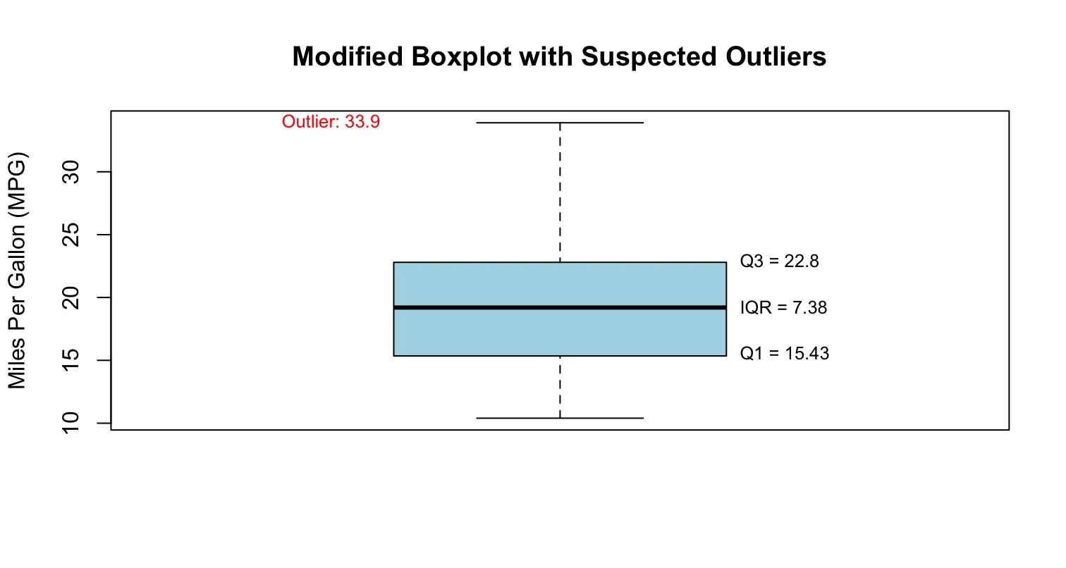
The interquartile range (IQR) is a measure of statistical dispersion, or spread, in a dataset. It is calculated as the difference between the third quartile (Q3) and the first quartile (Q1):
The IQR represents the range within which the central 50% of the data points lie. It is a robust measure of spread that is less affected by outliers compared to the range (which is the difference between the maximum and minimum values).
Rule for outliers: an observation N is considered a suspected outlier if:
- N > Q3 + 1.5 * IQR, or N < Q1 - 1.5 * IQR
- A modified boxplot is a boxplot with suspected outliers. R uses modified boxplots.
Example Code:
# Load the built-in dataset mtcars
data(mtcars)

# Extract the mpg (miles per gallon) variable
x <- mtcars$mpg

# Calculate quartiles and IQR
Q1 <- quantile(x, 0.25)   # First quartile (25th percentile)
Q3 <- quantile(x, 0.75)   # Third quartile (75th percentile)
IQR_value <- IQR(x)       # Interquartile range (Q3 - Q1)

# Define the lower and upper bounds for suspected outliers
lower_bound <- Q1 - 1.5 * IQR_value
upper_bound <- Q3 + 1.5 * IQR_value

# Identify suspected outliers
outliers <- x[x < lower_bound | x > upper_bound]

# Print results
cat("Q1 =", Q1, "\n")
cat("Q3 =", Q3, "\n")
cat("IQR =", IQR_value, "\n")
cat("Lower bound =", lower_bound, "\n")
cat("Upper bound =", upper_bound, "\n")
cat("Suspected outliers:", outliers, "\n")

# Create a modified boxplot (R automatically marks suspected outliers with dots)
boxplot(x,
        main = "Modified Boxplot with Suspected Outliers",
        ylab = "Miles Per Gallon (MPG)",
        col = "lightblue")

# Add labels for Q1, Q3, and IQR
text(x = 1.2, y = Q1, labels = paste0("Q1 = ", round(Q1, 2)), pos = 4, cex = 0.8)
text(x = 1.2, y = Q3, labels = paste0("Q3 = ", round(Q3, 2)), pos = 4, cex = 0.8)
text(x = 1.2, y = (Q1 + Q3) / 2, labels = paste0("IQR = ", round(IQR_value, 2)), pos = 4, cex = 0.8)

# Optionally add labels for outliers
if (length(outliers) > 0) {
  for (o in outliers) {
    text(x = 0.8, y = o, labels = paste("Outlier:", round(o, 1)), pos = 2, col = "red", cex = 0.8)
  }
}
# Output:
Q1 = 15.425
Q3 = 22.8
IQR = 7.375
Lower bound = 4.7875
Upper bound = 33.4375
Suspected outliers: 33.9
- There are different data types in programming. We’ve gone over several, like vectors, dataframes, matrices, etc.
- A string is a data type used to represent text.
Example:
x <- 27
mode(x)
y <- "27"
mode(y)
# Output:
[1] "numeric"
[1] "character"
The first example above shows x as a numeric vector, the second shows y as a character string.
- Concatenate 2 strings
str1 <- "Hello"
str2 <- "World"
result <- paste(str1, str2)
print(result)
# Output:
[1] "Hello World"
- Concatenate multiple strings
str1 <- "Data"
str2 <- "Science"
str3 <- "with"
str4 <- "R"
result <- paste(str1, str2, str3, str4)
print(result)
# Output:
[1] "Data Science with R"
- Concatenate strings with defined separator
str1 <- "10"
str2 <- "20"
str3 <- "2025"
date <- paste(str1, str2, str3, sep = "-")
print(date)
path = paste("home", "user", "documents", sep = "/")
print(path)
[1] "10-20-2025"
[1] "home/user/documents"
- nchar(): returns the number of characters in the given string
str <- "Hello, World!"
length <- nchar(str)
print(length)
# Output:
[1] 13
Note:
length(x) returns the number of elements in a vector, not the number of characters in a string. For a character vector containing a single string, length(x) returns 1. To count the number of characters in a string, use nchar(x).
Spaces are characters and are counted by nchar().
- substr(): returns the substring in the given position
str <- "Hello, World!"
sub_str <- substr(str, 8, 12)
print(sub_str)
substr(str, 1, 5)
substr(str, 8, 8)
# Output:
[1] "World"
[1] "Hello"
[1] "W"
- strsplit(): split the string with a given separator
str <- "apple,banana,cherry"
fruits <- strsplit(str, ",")
print(fruits)
# Output:
[[1]]
[1] "apple" "banana" "cherry"
- Using unlist() allows you to get a specific entry from y:
str <- "apple,banana,cherry"
fruits <- unlist(strsplit(str, ","))
fruits[2]
# Output:
[1] "banana"
str <- "apple,banana,cherry"
strsplit(str, "a")
# Output:
[[1]]
[1] "" "pple,b" "n" "n" ",cherry"
- grep(pattern, vector): returns the index of the string where pattern is a substring
fruits <- c("apple", "banana", "cherry", "date")
index <- grep("a", fruits)
print(index)
index <- grep("b", fruits)
print(index)
index <- grep("c", fruits)
print(index)
index <- grep("d", fruits)
print(index)
# Output:
[1] 1 2 4
[1] 2
[1] 3
[1] 4
When vector has only 1 element, grep() helps to determine whether the pattern is a substring.
str <- "Hello, World!"
index <- grep("World", str)
print(index)
index <- grep("world", str)
print(index)
# Output:
[1] 1
integer(0)
- regexpr(pattern, string): returns the first position of pattern if it’s a substring, returns -1 otherwise. regexpr stands for regular expression.
str <- "Hello, World!"
position <- regexpr("World", str)
print(position)
position <- regexpr("world", str)
print(position)
# Output:
[1] 8
attr(,"match.length")
[1] 5
attr(,"index.type")
[1] "chars"
attr(,"useBytes")
[1] TRUE
[1] -1
attr(,"match.length")
[1] -1
attr(,"index.type")
[1] "chars"
attr(,"useBytes")
[1] TRUE
- gregexpr(pattern, string): returns all starting positions if pattern is a substring, return -1 otherwise.
str <- "banana"
positions <- gregexpr("an", str)
print(positions)
positions <- gregexpr("na", str)
print(positions)
positions <- gregexpr("xy", str)
print(positions)
# Output:
[[1]]
[1] 2 4
attr(,"match.length")
[1] 2 2
attr(,"useBytes")
[1] TRUE
[[1]]
[1] 3 5
attr(,"match.length")
[1] 2 2
attr(,"useBytes")
[1] TRUE
[[1]]
[1] -1
attr(,"match.length")
[1] -1
attr(,"useBytes")
[1] TRUE
- sub(pattern, replacement, string): substitutes the pattern by the replacement at its first occurrence.
str <- "Hello, World! Welcome to the World of R."
new_str <- sub("World", "Universe", str)
print(new_str)
# Output:
[1] "Hello, Universe! Welcome to the World of R."
- gsub(pattern, replacement, string): substitutes the pattern by the replacement at ALL occurrences.
IMPORTANT NOTE: A pattern may be used in place of specific characters in this function.
str <- "Hello, World! Welcome to the World of R."
new_str <- gsub("World", "Universe", str)
print(new_str)
# Output:
[1] "Hello, Universe! Welcome to the Universe of R."
Also called regex. A regular expression is a string that describes a search pattern used to match text.
Key syntax and examples
- Character classes
-
[a-z]— any lowercase letter -
[A-Z]— any uppercase letter -
[0-9]or\d— any digit -
[a-zA-Z0-9]— any single alphanumeric character -
[^abc]— any character excepta,b, orc(negation inside brackets)
-
- Quantifiers
-
*— 0 or more occurrences (e.g.,(a)*matches"",a,aa, ...) -
+— 1 or more occurrences (e.g.,(a)+matchesa,aa, ...) -
?— 0 or 1 occurrence -
{n},{n,},{n,m}— exact or ranged repeats (e.g.,[0-9]{3}matches three digits)
-
- Anchors
-
^— start of string -
$— end of string - Example:
[a-z]*com$matches strings that end withcom
-
- Common tokens
-
\s— whitespace (space, tab, newline) -
\S— non-whitespace -
\w— word character (letter, digit, underscore) -
.— any character except newline (use.with care)
-
- Examples (simple)
-
CS[1-7][0-9]{2}— course codes likeCS158 -
[a-z0-9._%+-]+@[a-z0-9.-]+\.[a-z]{2,}— a basic email pattern (simplified) -
\s+— one or more whitespace characters
-
Notes for R
- R strings interpret backslashes, so patterns often need double escapes. Example: to match whitespace use
"\\s+"in R code. - Useful R functions:
-
grep(pattern, x)— indices of matches -
grepl(pattern, x)— logical vector (TRUE if match) -
regexpr(pattern, text)— position and length of first match -
gregexpr(pattern, text)— positions and lengths of all matches -
sub(pattern, replacement, text)— replace first match -
gsub(pattern, replacement, text)— replace all matches
-
R examples
texts <- c("user@example.com", "no-at-sign", "CS158")

# test for email-like strings (simplified)
grepl("[a-z0-9._%+-]+@[a-z0-9.-]+\\.[a-z]{2,}", texts, ignore.case = TRUE)

# find course codes
grep("^CS[1-7][0-9]{2}$", texts)

# replace whitespace with single space
gsub("\\s+", " ", "a\tb\nc")
# Output:
[1] TRUE FALSE FALSE
[1] 3
[1] "a b c"
Caveats
- Real-world email validation requires more complex rules than a simple regex.
- Behavior of
.and character classes may vary with flags (e.g., multiline, dotall). - Test patterns on representative inputs and consider edge cases.
Further reading
- Wikipedia: Regular expression (search "regular expression") or any regex tutorial for details and flavors.
Outline:
✅ 1. Introduction to R (Completed)
✅ 2. Getting Started with R (Completed)
✅ 3. Read/Write Files in R (Completed)
✅ 4. Control Flow (Completed)
✅ 5. Implicit Loops (Completed)
✅ 6. Plotting in R (Completed)
✅ 7. String Manipulation (Completed)
🟡 8.Statistical Analysis (Upcoming)
🔜 ❓ TBD (To Be Determined)
❓Writing Custom Functions
❓Package Development (Advanced)
(Some of these issues may be closed or open/in progress.)
Xuye Luo
https://posit.co/download/rstudio-desktop
https://github.com/imtiaz-emu/Data-Science-with-R
https://www.geeksforgeeks.org/r-language/apply-lapply-sapply-and-tapply-in-r/#