-
Notifications
You must be signed in to change notification settings - Fork 28
First steps
#First steps
The basic functionality of the software that loads, links, plots and fits model and data will be explained.
In the folder /Examples we provide some showcase applications that can be used as a starting point for new modeling projects.
Once models and data have been implemented in the current working directory (in subfolders /models and /data) models and data can be loaded, compiled and linked. A typical MATLAB script would look like this
arInit;

arLoadModel('model1', 1);
arLoadModel('model2', 2);

arLoadData('data1_for_model1', 1);
arLoadData('data2_for_model1', 1);
arLoadData('data3_for_model2', 2);
arLoadData('data4_for_model2', 2);

arCompileAll;
After the setup script finished successfully full functionality can be used. All information about model and data are now available in the global variable ar. Below some basic function are explained briefly.
Basic commands / functions
Displays the list of all model parameters, their current values, upper bound (ub) and lower bound (lb), ... in the MATLAB command window.
Parameters: # = free, C = constant, D = dynamic, I = initial value, E = error model

           name                       lb       value       ub          10^value        fitted   prior
#   1|DI | CISEqc                   |       -3       +2.6         +4 | 1   +4.3e+02 |       1 | uniform(-3,4)
#   2|DI | CISEqcOE                 |       -3      -0.28         +3 | 1      +0.53 |       1 | uniform(-3,3)
#   3|D  | CISInh                   |       -3       +8.9        +12 | 1   +7.9e+08 |       1 | uniform(-3,12)
...
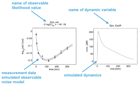
Opens plots of the model trajectories and of the experimental data for the current parameter values.

arPlotter opens a small graphical user interface that allows select with data sets and available quantities to display by arPlot command.
Runs the currently selected numerical optimization algorithm to calibrate the model to the experimental data. Maximum likelihood estimation is used here. If the the option flag in the global variable ar.config.showFitting = true the process of the model calibration is shown during the estimation (see arPlot).
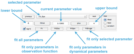
Opens a small graphical user interface that allows to manually adjust parameter values and updates the corresponding plots (see arPlot).

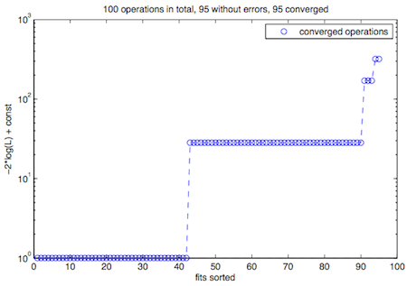
Executes a sequence of n fits (see arFit). For deterministic optimization the initial parameter guesses are generated by Latin hypercube sampling (LHS). The results of the n fits are displayed by arPlotFits sorted by goodness of fit and the parameter values of the best fit replace the previous values.

- Installation and system requirements
- Setting up models
- First steps
- Advanced events and pre-equilibration
- Computation of integration-based prediction bands
- How is the architecture of the code and the most important commands?
- What are the most important fields of the global variable ar?
- What are the most important functions?
- Optimization algorithms available in the d2d-framework
- Objective function, likelhood and chi-square in the d2d framework
- How to set up priors?
- How to set up steady state constraints?
- How do I restart the solver upon a step input?
- How to deal with integrator tolerances?
- How to implement a bolus injection?
- How to implement washing and an injection?
- How to implement a moment ODE model?
- How to run PLE calculations on a Cluster?